Patterns of functional vision loss in glaucoma determined with archetypal analysis

Abstract

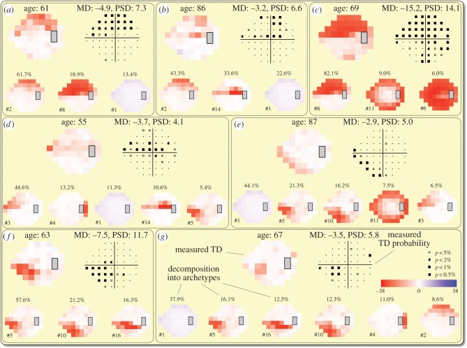
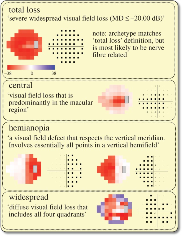
Glaucoma is an optic neuropathy accompanied by vision loss which can be mapped by visual field (VF) testing revealing characteristic patterns related to the retinal nerve fibre layer anatomy. While detailed knowledge about these patterns is important to understand the anatomic and genetic aspects of glaucoma, current classification schemes are typically predominantly derived qualitatively. Here, we classify glaucomatous vision loss quantitatively by statistically learning prototypical patterns on the convex hull of the data space. In contrast to component-based approaches, this method emphasizes distinct aspects of the data and provides patterns that are easier to interpret for clinicians. Based on 13 231 reliable Humphrey VFs from a large clinical glaucoma practice, we identify an optimal solution with 17 glaucomatous vision loss prototypes which fit well with previously described qualitative patterns from a large clinical study. We illustrate relations of our patterns to retinal structure by a previously developed mathematical model. In contrast to the qualitative clinical approaches, our results can serve as a framework to quantify the various subtypes of glaucomatous visual field loss.

Keywords: glaucoma; retinal nerve fibre layer; vision loss.

Figure 1.

Comparison of the two approaches of unsupervised statistical learning procedures applied to VFs. (a,c) The prototype approach tries to partition the data. Each partition can be characterized by a representative pattern (prototype). The simple two-dimensional example in (a) illustrates this by a cluster analysis algorithm (k-means) applied to two-dimensional data. The component approach (b,d) tries to identify hidden structure or components of the data, typically by axes, as illustrated in (b) by principal component analysis. (c,d) Apply the algorithms of the two-dimensional examples to our 52-dimensional VF data.

Figure 2.

Illustration of statistical learning algorithms by simple two-dimensional examples. (a) Principal component analysis (PCA), independent component analysis (ICA) and archetypal analysis (AA) applied to a non-Gaussian random set of points. Unlike the orthogonal PCA axes (dashed lines), the non-orthogonal ICA axes (solid lines) cover the two independent sources of the dataset. PCA and ICA represent directions in the data space, but do not define representative patterns. By contrast, the four archetypes defined by AA (asterisks) place representative patterns on the convex hull of the data space. (b) Variational Bayesian ICA (vB-ICA) combines clustering with the component approach. ICA is applied to each cluster separately. (Online version in colour.)

Figure 3.

The five vB-ICA axes of the moderate-to-severe cluster from Goldbaum et al. [19]. The colour plots show the total deviations in dB at ±2 standard deviations (s.d.) from the cluster centroid for each of the five ICA axes. The descriptions of the patterns are adapted from table 2 in [19] (inf., inferior; sup., superior).

Figure 4.

Mean deviations versus pattern standard deviations of all VF measurements. Distributions are illustrated by marginal histograms. Quartiles are annotated. (Online version in colour.)

Figure 5.

Tenfold cross-validation of archetypal analysis. The y-axis shows the residual sum of squares (RSS) normalized by number of samples. The black circles denote the RSS values for each of the 10 testing partitions for each number of archetypes. The black line connects their medians. The plus symbols denote the differences of the Bayesian information criteria (BIC) between a linear model with a local slope ≠ 0 and a ‘null model’ of a horizontal line (see §2.2). A BIC difference above 0 (dashed line) indicates preference of the null model, that is, the local slope is not different from 0. (Online version in colour.)

Figure 6.

The optimal solution with 17 archetypes. The archetypes are sorted decreasingly by their relative weights in the dataset. The colours denote total deviations (differences of thresholds from age-specific normal values in dB; red, thresholds below norm; blue, threshold above norm). The numerical values of the archetypes are provided as the electronic supplementary material.

Figure 7.

Decomposition of a VF into archetypes and reconstruction. An illustrative VF of a 42-year-old open angle glaucoma (OAG) patient (a) is decomposed into the 17 archetypes (b). The archetype indices, denoted by AT, are the same as in figure 6. Only four archetypes (#6, #9, #10, and #11) have substantial coefficients. The other 13 archetypes have coefficients below 0.01% and are negligible for this VF. Finally, the original VF is reconstructed by calculating a weighted sum of the archetypes and their coefficients (c). (Online version in colour.)

Figure 8.

Illustrative examples of VF measurements and their decompositions into archetypes. Top row in each box: total deviation (TD, in dB) and TD probability plots of respective measurement. Bottom row: archetypes and their coefficients, sorted in decreasing order. Only archetypes with coefficients ≥5% are shown. To the bottom left or each archetype, the index from figure 6 is denoted. (a–d) Predominantly upper hemifield defects; (e–g) predominantly lower hemifield defects. MD, mean deviation in dB; PSD, pattern standard deviation. The VF measurements are not from the dataset that was used for statistically learning the archetypes.

Figure 9.

Archetypes that match nerve fibre-related defects of the ocular hypertension treatment study (OHTS). Categories and their verbal descriptions from [7]. Colour plots: total deviation (TD; in dB). To the right of each TD plot, the TD probability plot is shown (see legend in figure 7 for the meaning of the black symbols).

Figure 10.

Archetypes that match non-nerve fibre-related defects of the ocular hypertension treatment study (OHTS). Categories and their verbal descriptions from [7]. See caption of figure 9 for details.

Figure 11.

Characteristics of predominantly lower hemifield nerve fibre-related archetypes. Total deviations (TDs, in dB), TD probability plots (see legend in figure 7 for the meaning of the black symbols), and modelled nerve fibre defects of each nerve fibre-related archetype that predominantly affects the lower visual hemifield, together with two respective illustrative examples of measured VFs. MD and PSD refer to mean deviation (in dB) and pattern standard deviation of the archetype. Age refers to patient age at the time of the respective VF measurement. AT coeff. denotes the coefficient of the respective archetype for the measured VF. The nerve fibre model plots are centred around the fovea (denoted by F). The grey disc illustrates the optic nerve head (ONH). RNFL maps are mirrored at the horizon relative to VFs according to conventions used in ophthalmology. (Online version in colour.)

Figure 12.

Characteristics of predominantly upper hemifield nerve fibre-related archetypes. See caption of figure 11 for details. (Online version in colour.)

Figure 13.

Characteristics of annular nerve fibre-related archetypes. See caption of figure 11 for details. (Online version in colour.)

Figure 14.

Characteristics of the temporal nerve fibre-related archetype. See caption of figure 11 for details. (Online version in colour.)

References

1. Quigley HA. 2011. Glaucoma. Lancet 377, 1367–1377. (10.1016/S0140-6736(10)61423-7) - DOI - PubMed
1. Brusini P, Johnson CA. 2007. Staging functional damage in glaucoma: review of different classification methods. Surv. Ophthalmol. 52, 156–179. (10.1016/j.survophthal.2006.12.008) - DOI - PubMed
1. Wiggs JL, et al. 2012. The p53 codon 72 PRO/PRO genotype may be associated with initial central visual field defects in Caucasians with primary open angle glaucoma. PLoS ONE 7, e45613 (10.1371/journal.pone.0045613) - DOI - PMC - PubMed
1. Loomis SJ, et al. 2014. Association of cav1/cav2 genomic variants with primary open-angle glaucoma overall and by gender and pattern of visual field loss. Ophthalmology 121, 508–516. (10.1016/j.ophtha.2013.09.012) - DOI - PMC - PubMed
1. Buys ES, et al. 2013. Soluble guanylate cyclase 1-deficient mice: a novel murine model for primary open angle glaucoma. PLoS ONE 8, e60156 (10.1371/journal.pone.0060156) - DOI - PMC - PubMed
Publication types
LinkOut - more resources