Stochastic simulation in systems biology

Abstract

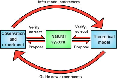
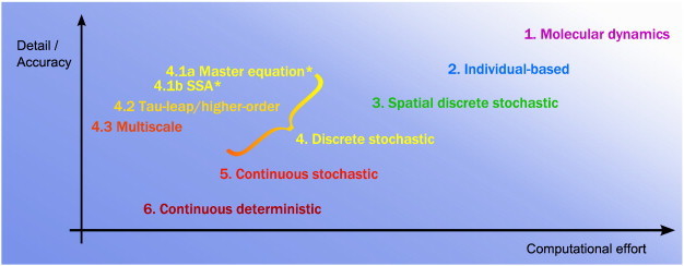
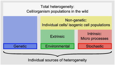
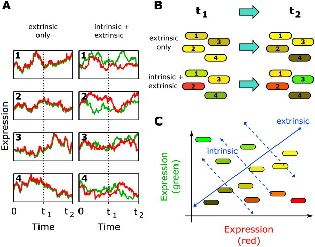
Natural systems are, almost by definition, heterogeneous: this can be either a boon or an obstacle to be overcome, depending on the situation. Traditionally, when constructing mathematical models of these systems, heterogeneity has typically been ignored, despite its critical role. However, in recent years, stochastic computational methods have become commonplace in science. They are able to appropriately account for heterogeneity; indeed, they are based around the premise that systems inherently contain at least one source of heterogeneity (namely, intrinsic heterogeneity). In this mini-review, we give a brief introduction to theoretical modelling and simulation in systems biology and discuss the three different sources of heterogeneity in natural systems. Our main topic is an overview of stochastic simulation methods in systems biology. There are many different types of stochastic methods. We focus on one group that has become especially popular in systems biology, biochemistry, chemistry and physics. These discrete-state stochastic methods do not follow individuals over time; rather they track only total populations. They also assume that the volume of interest is spatially homogeneous. We give an overview of these methods, with a discussion of the advantages and disadvantages of each, and suggest when each is more appropriate to use. We also include references to software implementations of them, so that beginners can quickly start using stochastic methods for practical problems of interest.

Keywords: Discrete-state stochastic methods; Heterogeneity; Stochastic simulation.

Fig. 1

Illustration of the cycle of information flow between the natural world and our theoretical and experimental efforts to understand it.

Fig. 2

Modelling and simulation methods compared based on their level of detail/accuracy versus their computational difficulty. We focus on the fourth category of methods, which we have broken down into sub-categories that we describe in Section 5. The figure is not to scale. *The master equation and the SSA are both ‘exact’ as such (see Section 5), but there are some caveats. The master equation can be solved exactly, numerically or by approximations, whilst the SSA is strictly only exact in the limit of infinite simulations.

Fig. 3

Sources of heterogeneity. The total observed heterogeneity in a natural system broken down into its three components: genetic, environmental, and stochastic. Different sources of heterogeneity are present at different scales, and the typical scales are given.

Fig. 4

Separating intrinsic and extrinsic noise with a two-colour experiment. Here we illustrate the classic two-colour experiment of Elowitz et al. . Two differently-coloured fluorescent proteins (here, red and green) are inserted into the genome of E. coli. (A) Hypothetical time series of fluorescent protein expression for either extrinsic noise only (correlated expression), or both intrinsic and extrinsic noise (uncorrelated expression). Numbers are labels for each bacterial cell. (B) The corresponding population-level view of the bacterial cells at each of the two time points t₁ and t₂. (C) Plotting the expression levels of the fluorescent proteins on the same figure, extrinsic noise results in variation along the diagonal (blue line). Intrinsic noise results in deviations from the diagonal (dashed blue lines).

Fig. 5

Simulations of the Schlögl system using deterministic and stochastic methods. Four typical trajectories of the SSA (coloured lines, left panels) and ordinary differential equations (black lines, left panels). The full distribution at simulation time T = 10, in the limit of a large number of simulations, is shown in the right panels for each initial configuration. Note that here we actually used the master equation (see Section 5), which can be solved numerically for this problem, to generate these as it allowed for faster computation. Parameters used are A = 10⁵, B = 2 × 10⁵ and c₁ = 3 × 10^− 7, c₂ = 10^− 4, c₃ = 10^− 3, and c₄ = 3.5.

Fig. 6

Comparison of simulation methods. (A) Two typical trajectories each from the SSA (green line) and tau-leap (red dotted line) and ordinary differential equation solutions (black line). The inset shows an enlargement between t = 6.7 and t = 6.9 to highlight the discrete steps of the SSA. (B) Full probability distributions at final time T = 10 generated from 10⁴ simulations of the SSA and tau-leap with step sizes 0.05 and 0.4, compared to the solution of the master equation (from which the SSA is almost indistinguishable). Here X(0) = 250.

References

-
- Mitchell M. Oxford University Press; New York, NY: 2009. Complexity: a guided tour.
- Kitano H. Computational systems biology. Nature. 2002;420:206–210. - PubMed
- Epstein J.M. Why model? J Artif Soc Soc Simul. 2008;11:12.
Publication types
LinkOut - more resources
Full Text Sources
Other Literature Sources