Spatial genome organization: contrasting views from chromosome conformation capture and fluorescence in situ hybridization

Abstract

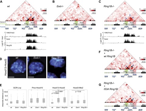
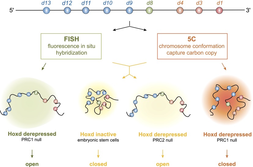
Although important for gene regulation, most studies of genome organization use either fluorescence in situ hybridization (FISH) or chromosome conformation capture (3C) methods. FISH directly visualizes the spatial relationship of sequences but is usually applied to a few loci at a time. The frequency at which sequences are ligated together by formaldehyde cross-linking can be measured genome-wide by 3C methods, with higher frequencies thought to reflect shorter distances. FISH and 3C should therefore give the same views of genome organization, but this has not been tested extensively. We investigated the murine HoxD locus with 3C carbon copy (5C) and FISH in different developmental and activity states and in the presence or absence of epigenetic regulators. We identified situations in which the two data sets are concordant but found other conditions under which chromatin topographies extrapolated from 5C or FISH data are not compatible. We suggest that products captured by 3C do not always reflect spatial proximity, with ligation occurring between sequences located hundreds of nanometers apart, influenced by nuclear environment and chromatin composition. We conclude that results obtained at high resolution with either 3C methods or FISH alone must be interpreted with caution and that views about genome organization should be validated by independent methods.

Keywords: 3C; FISH; Hox genes; nuclear organization; polycomb.

Figure 1.

5C analysis of HoxD in ESCs. (A) A 670-kb region analyzed by 5C in OS25 mESCs, encompassing Mtx2, Hoxd genes, Evx2, and Lnp. Distal regulatory elements (Montavon et al. 2011) are highlighted in green. Positions of FISH probes are indicated in blue. Genome coordinates are from the NCBI37/mm9 assembly of the mouse genome. (B) Analysis of chromatin organization in undifferentiated mESCs by 5C sequencing across the 670-kb region shown in A. The heat map shows 5C data binned over 20-kb windows. Heat map intensities represent the average of interaction frequency for each window, color-coded according to the scale shown. Data for a biological replicate are in Supplemental Figure S1A. Unprocessed normalized data are shown in Supplemental Figure S7. All interaction frequencies were first normalized based on the total number of sequence reads in the 5C data set. (C) High-resolution (12-kb binning) zoomed-in view of the 5C data over Exv2 and the HoxD locus. The two contacts conserved in human embryonic carcinoma cells are indicated with dashed yellow boxes. (D) Two-dimensional schematic interpretation of the 5C data in OS25 mESCs illustrating the folded nature of the Evx2–HoxD domain (not to scale). Contacts between Hoxd11 and regions downstream from d1, d3, and Evx2 are highlighted in yellow.

Figure 2.

Decompaction of the HoxD cluster and increased long-range interactions accompany ESC differentiation. (A) Analysis of chromatin organization during OS25 mESC differentiation by 5C sequencing across a 670-kb region containing Lnp, Evx2, HoxD genes, and Mtx2 in undifferentiated ESCs (left) and differentiated cells (D3; right). Blue arrows point to GCR–Lnp contacts and HoxD contacts to compare interaction frequencies. The top heat maps show 5C data binned over 20-kb windows, and heat map intensities represent the average interaction frequency for each window. Interaction frequencies were normalized based on total sequence read number. Yellow shading indicates the region of strong 5C signals. H3K27me3 ChIP–chip data (Eskeland et al. 2010) are presented below. The bottom left heat map shows Hi-C data at 30-kb resolution, normalized based on read depth (Dixon et al. 2012), and TADs for the corresponding region in mESCs. Data for a biological replicate are in Supplemental Figure S1. Unprocessed normalized data are shown in Supplemental Figure S6A. (B) Heat map showing interactions enriched in D3 differentiated (red) or undifferentiated (blue) ESCs. Heat map values represent the difference of normalized interaction frequencies between D3 differentiated and undifferentiated cells as indicated by the color scale at the right. Green and red shading highlight the regions covered by the fosmids used for the analysis in C. (C) 3D-FISH with Hoxd13 and Hoxd3 probe pairs counterstained with DAPI (blue) in nuclei from undifferentiated (Undiff) and differentiated (D3) ESCs. Bars, 5 μm. (D) Box plots showing the distribution of squared interprobe distances (d²) in micrometers for GCR–Lnp, Prox–Hoxd10, Hoxd13–Hoxd3, Hoxd3–Mtx2P, and Mtx2P–3′Mtx2 FISH probe pairs in undifferentiated (left) and D3 (middle) mESCs. The right box plots compare the interprobe distance distributions for each probe pair in undifferentiated (Undiff) versus D3 ESCs. Boxes show the median and interquartile range of the data; crosses signify outliers. n = 86–101 loci. The statistical significance between data sets was examined by Mann-Whitney U-tests. These data are plotted as histograms of the frequency distribution in Supplemental Figure S2.

Figure 3.

FISH analysis of the 5′ HoxD regulatory region in anterior and posterior distal limb cells. (A) A 1.16-Mb region analyzed by 5C in limb cells and including the gene desert 5′ of HoxD that contains distal limb-specific regulatory elements (highlighted in green) (Montavon et al. 2011). Positions of the fosmids used for FISH experiments are indicated in blue. (B) FISH with Hoxd13 and GCR probes in nuclei of cell lines derived from the anterior (A2) or posterior (P2) E10.5 distal embryonic forelimb (left) and anterior or posterior E11.0 distal forelimb tissue (right). Bars, 5 μm. (C) Frequency distributions of interprobe distances (d) in 0.2-μm bins between the GCR, Hoxd13, and IslIII probes in nuclei from A2 and P2 limb cell lines (left) or anterior (A) and posterior (P) parts of the distal E11.0 forelimb bud (right) (data from Williamson et al. 2012). n = 93–151. Error bars represent SEM obtained from two different tissue sections. (D) Box plots below show the distribution of squared interprobe distances (d²) in micrometers between IslIII/Hoxd13, IslIII/GCR, and GCR/Hoxd13 probe pairs in A2 and P2 limb cell lines (left) and anterior (A) or posterior (P) limb tissue (right). n = 191 loci for cell lines; n = ∼100 loci for tissue. The statistical significance of differences between data from distal anterior and distal posterior nuclei was examined by Mann-Whitney U-tests.

Figure 4.

Long-range interactions in the 5′ HoxD regulatory region in anterior and posterior distal limbs. (A) 5C heat maps show the average interaction frequencies (24-kb bins) across HoxD and its regulatory domain in anterior (A2; top) and posterior (P2; bottom) limb cell lines according to color scales as described in Figure 1. Interaction frequencies were normalized based on total sequence read number. Black dotted lines indicate the areas encompassing IslIII–Hoxd13 or GCR–Hoxd13. (B, top) Heat map showing 5C interactions enriched in P2 (red) or A2 (blue) cells. Heat map values are the difference of normalized interaction frequencies between P2 and A2 cells and are color-coded according to the scale at the top right. (Bottom) Heat map shows Hi-C data normalized based on read depth and the position of TADs (Dixon et al. 2012) for the corresponding region in mESCs. (C) Virtual 4C analysis obtained by extracting 5C interactions with viewpoints fixed at IslIII, GCR, Hoxd13, Hoxd9–10, and Hoxd1. Dashed lines indicate the position of the fixed viewpoint from regulatory elements (green) or Hoxd genes (orange). Data from A2 anterior and P2 posterior limb cell lines are in open and filled circles, respectively. Data from a biological replicate are shown in Supplemental Figure S4, and unprocessed normalized data are shown in Supplemental Figure S6B.

Figure 5.

5C signals within the HoxD domain in polycomb mutant ESCs. 5C sequencing across HoxD in wild-type (wt) (A), PRC2 mutant (Eed^−/−) (B), and PRC1 mutant (Ring1B^−/−) (C) mESCs. 5C heat maps show the average interaction frequencies, normalized based on total sequence read number, per 20-kb bin using color scales as described in Figure 1. Below the heat maps, the position of genes is indicated in gray, regulatory elements are in green, and fosmid probes are in blue. Green and red highlight the regions covered by the fosmids used for the analysis in D. In A and C, ChIP–chip data for H3K27me3, Ezh2 (PRC2), and Ring1B (PRC1) from the respective mESCs are shown below the 5C heat maps (data from Illingworth et al. 2012). In Eed^−/− ESCs, Ezh2 is degraded, and H3K27me3 is reduced globally (Montgomery et al. 2005), so no ChIP data are shown. Data for a biological replicate are in Supplemental Figure S5. Unprocessed normalized data are shown in Supplemental Figure S7A. (D) 3D-FISH with Hoxd13 and Hoxd3 probe pairs (red and green) in nuclei (blue) from wild-type (wt) and polycomb-null mutant (Eed^−/− and Ring1B^−/−) mESCs. Bars, 5 μm. (E) Box plots showing the distribution of 3D-FISH squared interprobe distances (d²) for probe pairs GCR–Lnp, Prox–Hoxd10, Hoxd13–Hoxd3, and Hoxd3–Mtx2P in wild-type and polycomb-null mutant (Eed^−/− and Ring1B^−/−) ESCs. Boxes show the median and interquartile range of the data; crosses signify outliers. n = 93–107 loci. The statistical significances between the probe pairs covering the same region in different cells were examined by Mann-Whitney U-tests. (F,G) 5C sequencing across HoxD in Ring1B^−/− mESCs rescued with wild-type Ring1B (F) and I53A mutant Ring1B (G) (Eskeland et al. 2010). 5C heat maps show the mean interaction frequencies per 20-kb bin. Data for a biological replicate are in Supplemental Figure S5. Unprocessed normalized data are shown in Supplemental Figure S7B.

Figure 6.

FISH and 5C analysis can yield compatible or discordant chromatin topographies at high resolution. (Top) Schematic of the HoxD locus showing the 5′ (blue) and 3′ (orange) Hoxd genes. (Bottom) The views of chromatin topography for HoxD extrapolated from FISH or 5C data are shown for wild-type and polycomb mutant ESCs. (Middle) For wild-type and PRC2-null cells, FISH and 5C give coherent views of a compact (wild-type) versus unfolded (PRC2-null) chromatin conformation. However, in the case of PRC1-null cells, FISH (left) indicates an unfolded chromatin conformation similar to that seen for PRC2-null cells, whereas 5C (right) suggests a much more tightly folded domain.

References

1. Albiez H, Cremer M, Tiberi C, Vecchio L, Schermelleh L, Dittrich S, Küpper K, Joffe B, Thormeyer T, von Hase J, et al. . 2006. Chromatin domains and the interchromatin compartment form structurally defined and functionally interacting nuclear networks. Chrom Res 14: 707–733. - PubMed
1. Amano T, Sagai T, Tanabe H, Mizushina Y, Nakazawa H, Shiroishi T. 2009. Chromosomal dynamics at the Shh locus: limb bud-specific differential regulation of competence and active transcription. Dev Cell 16: 47–57. - PubMed
1. Andrey G, Montavon T, Mascrez B, Gonzalez F, Noordermeer D, Leleu M, Trono D, Spitz F, Duboule D. 2013. A switch between topological domains underlies HoxD genes collinearity in mouse limbs. Science 340: 1234167. - PubMed
1. Azuara V, Perry P, Sauer S, Spivakov M, Jørgensen HF, John RM, Gouti M, Casanova M, Warnes G, Merkenschlager M, et al. . 2006. Chromatin signatures of pluripotent cell lines. Nat Cell Biol 8: 532–538. - PubMed
1. Baù D, Marti-Renom MA. 2011. Structure determination of genomic domains by satisfaction of spatial restraints. Chrom Res 19: 25–35. - PubMed
Publication types