

A systematic framework for functional connectivity measures
- PMID: 25538556
- PMCID: PMC4260483
- DOI: 10.3389/fnins.2014.00405
A systematic framework for functional connectivity measures
Abstract
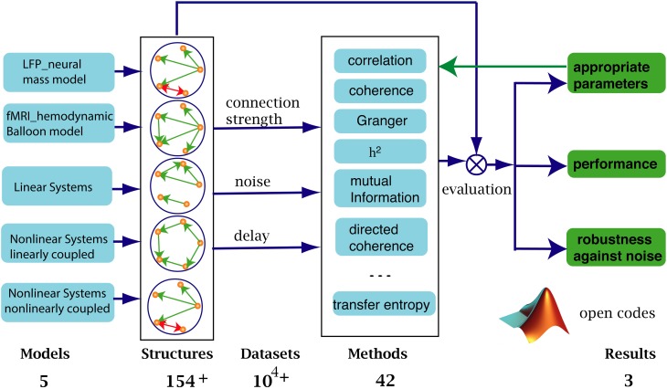
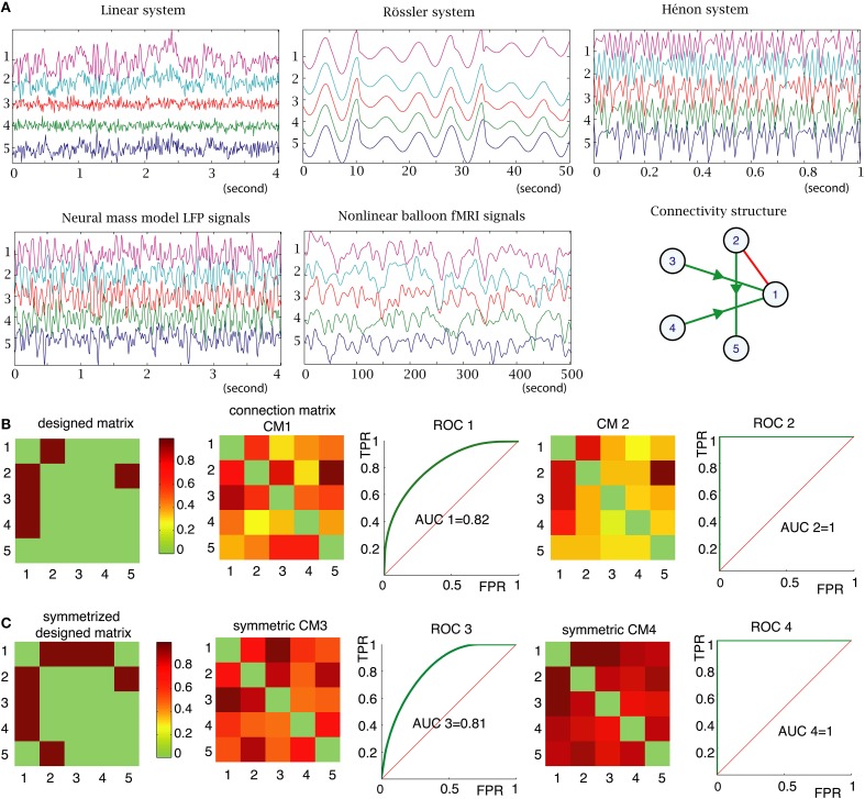
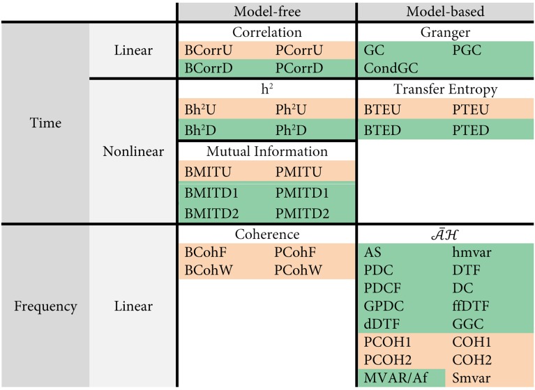
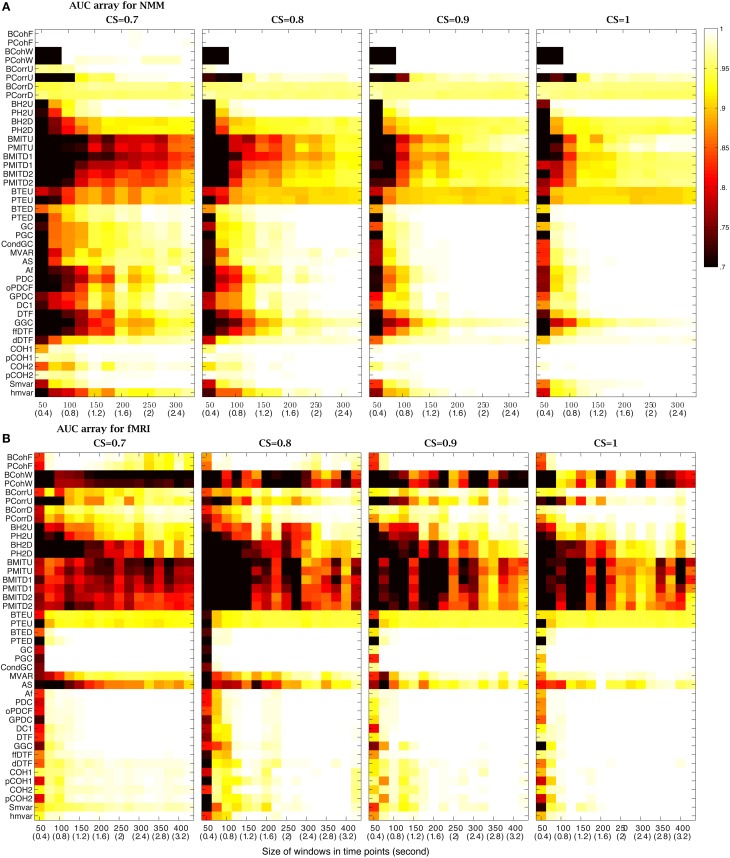
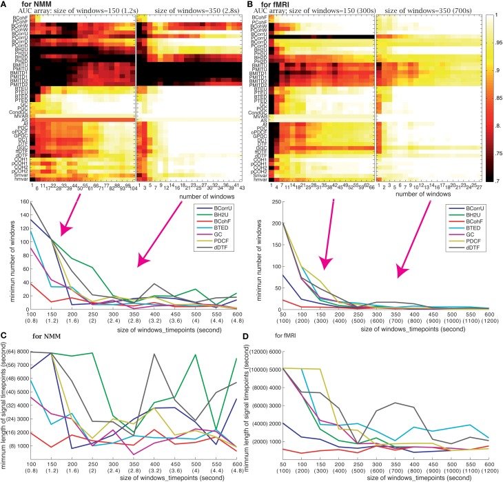
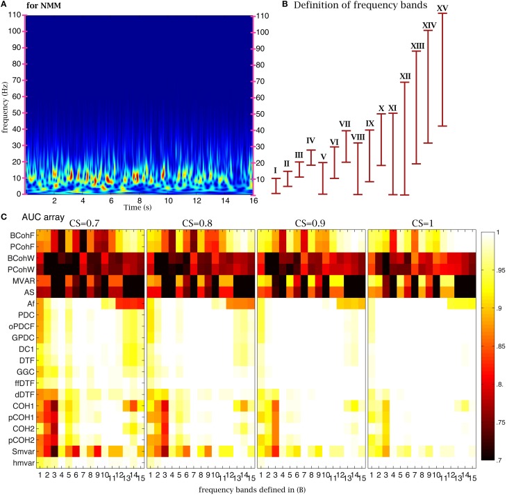
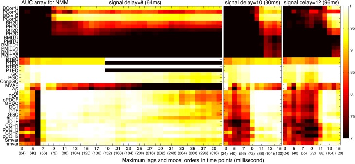
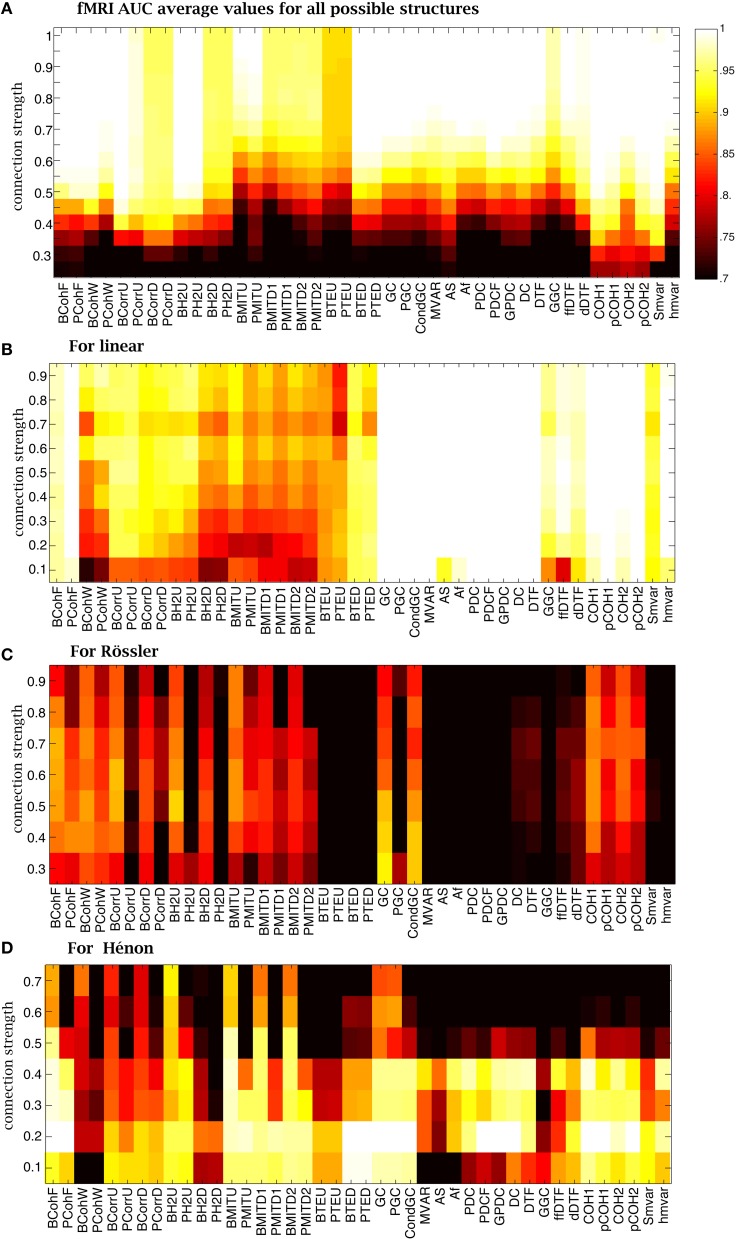
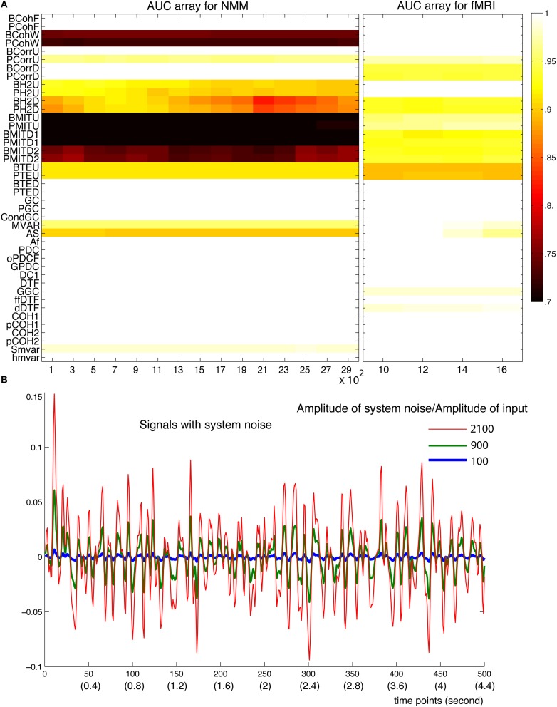
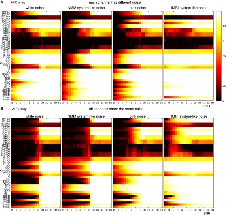
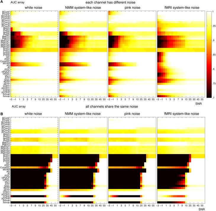
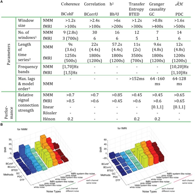
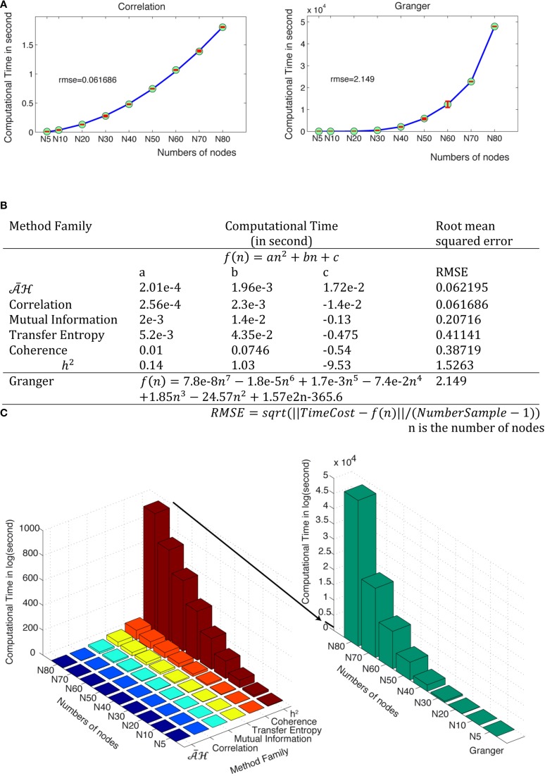
Various methods have been proposed to characterize the functional connectivity between nodes in a network measured with different modalities (electrophysiology, functional magnetic resonance imaging etc.). Since different measures of functional connectivity yield different results for the same dataset, it is important to assess when and how they can be used. In this work, we provide a systematic framework for evaluating the performance of a large range of functional connectivity measures-based upon a comprehensive portfolio of models generating measurable responses. Specifically, we benchmarked 42 methods using 10,000 simulated datasets from 5 different types of generative models with different connectivity structures. Since all functional connectivity methods require the setting of some parameters (window size and number, model order etc.), we first optimized these parameters using performance criteria based upon (threshold free) ROC analysis. We then evaluated the performance of the methods on data simulated with different types of models. Finally, we assessed the performance of the methods against different levels of signal-to-noise ratios and network configurations. A MATLAB toolbox is provided to perform such analyses using other methods and simulated datasets.
Keywords: Granger causality; evaluation framework; fMRI; functional connectivity; neural mass models.
Figures

 families).
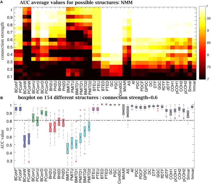
References
-
- Baccalá L. (2007). Generalized partial directed coherence, in Digital Signal Processing, 2007 15th International Conference on (Baccald, LA: IEEE; ), 163–166 10.1109/ICDSP.2007.4288544 - DOI
-
- Baccalá L., Sameshima K., Ballester G., Do Valle A. C., Timo-loria C. (1998). Studying the interaction between brain structures via directed coherence and Granger causality. Appl. Signal Process. 5, 40–48 10.1007/s005290050005 - DOI
-
- Baccalá L., Takahashi D., Sameshima K. (2006). Computer intensive testing for the influence between time series, in Handbook of Time Series Analysis, eds Schelter B., Winterhalder M., Timmer J. (Weinheim: Wiley-VCH; ), 411.
Grants and funding
LinkOut - more resources
Full Text Sources
Other Literature Sources