Dynamics of nutrient uptake strategies: lessons from the tortoise and the hare

Abstract

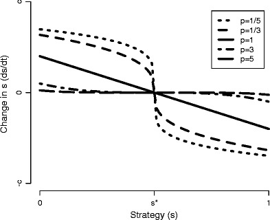
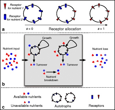
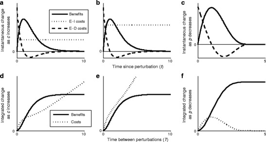
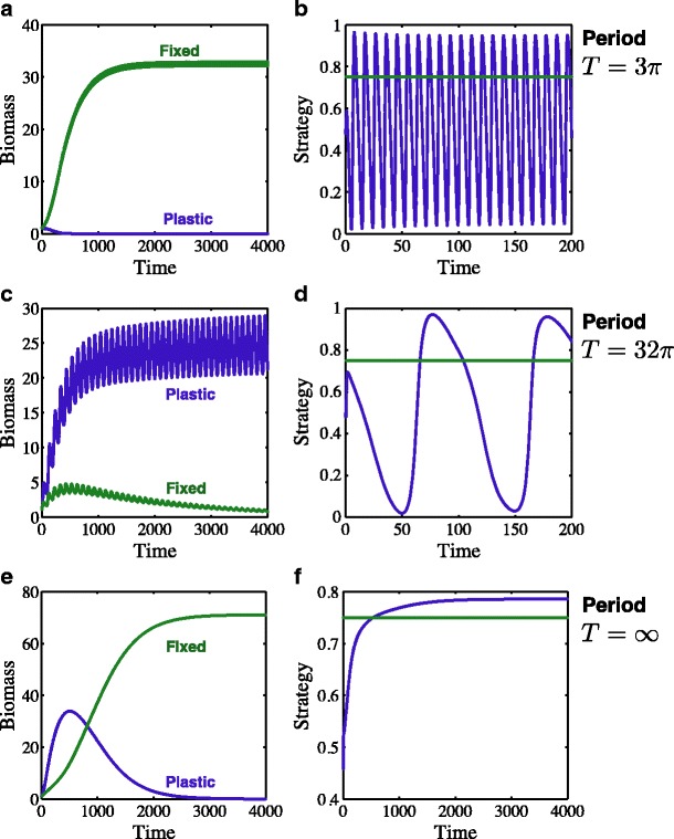
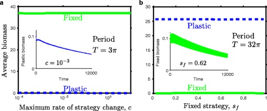
Many autotrophs vary their allocation to nutrient uptake in response to environmental cues, yet the dynamics of this plasticity are largely unknown. Plasticity dynamics affect the extent of single versus multiple nutrient limitation and thus have implications for plant ecology and biogeochemical cycling. Here we use a model of two essential nutrients cycling through autotrophs and the environment to determine conditions under which different plastic or fixed nutrient uptake strategies are adaptive. Our model includes environment-independent costs of being plastic, environment-dependent costs proportional to the rate of plastic change, and costs of being mismatched to the environment, the last of which is experienced by both fixed and plastic types. In equilibrium environments, environment-independent costs of being plastic select for tortoise strategies-fixed or less plastic types-provided that they are sufficiently close to co-limitation. At intermediate levels of environmental fluctuation forced by periodic nutrient inputs, more hare-like plastic strategies prevail because they remain near co-limitation. However, the fastest is not necessarily the best. The most adaptive strategy is an intermediate level of plasticity that keeps pace with environmental fluctuations, but is not faster. At high levels of environmental fluctuation, the environment-dependent cost of changing rapidly to keep pace with the environment becomes prohibitive and tortoise strategies again dominate. The existence and location of these thresholds depend on plasticity costs and rate, which are largely unknown empirically. These results suggest that the expectations for single nutrient limitation versus co-limitation and therefore biogeochemical cycling and autotroph community dynamics depend on environmental heterogeneity and plasticity costs.Electronic supplementary material The online version of this article (doi:10.1007/s12080-010-0110-0) contains supplementary material, which is available to authorized users.

Keywords: Biogeochemistry; Co-limitation; Dynamics; Ecosystem theory; Nutrient limitation; Plasticity; Strategies.

Fig. 1

Rate of change of the strategy s in response to distance from co-limitation (s ^* − s), as defined in Eq. 2. The strategy s is defined as the proportion of effort devoted to acquiring nutrient 1, so it varies from 0 to 1. The value s ^* is the co-limitation point, which is a function of the nutrient concentrations (see Eq. 7) so it changes through time. In this figure, s ^* is 0.5. The parameter c is the maximum absolute rate of change, realized for s = 0, s ^* = 1 or vice versa for each p. The curves are Eq. 2 with different values of p: p < 1 is concave downward to the left of s ^*, p = 1 is linear, and p > 1 is concave upward to the left of s ^*

Fig. 2

Cartoon diagram of the model. a The strategy (Fig. 1) is defined by the proportion of effort allocated to acquiring nutrient 1. The circles depict autotroph uptake areas, such as root surface area for higher plants or cell surface area for unicellular phytoplankton. b, c The model ecosystem consists of two nutrients cycling through autotroph biomass and the environment. Nutrients in the environment exist in forms that are unavailable and available to the autotroph. Autotroph growth and nutrient uptake depend on whichever nutrient is more limiting, which itself is affected by the strategy. Because of plasticity costs, the nutrient uptake strategy also affects autotroph turnover/mortality, which returns nutrients to the environment. Unavailable nutrients are broken down into available nutrients and can also be lost from the system. Available nutrients can be taken up or lost from the system and come from an external source as well as the decomposition of unavailable nutrients. Multiple autotroph types interact with each other solely through their effects on nutrients in the environment

Fig. 3

Benefits and costs of plasticity. Top panels show instantaneous benefits (due to being nearer co-limitation), environment-independent (E-I) costs (due to increased detection infrastructure), and environment-dependent (E-D) costs (due to more rapid changing of the strategy) of increasing plasticity as a function of time since a perturbation. Bottom panels show the integrated benefits and costs of increasing plasticity as a function of time between perturbations, i.e., integrated to a particular point on the horizontal axis in the top panel. Panels show effects of increasing c for low (a, d) and high (b, e) E-I costs and decreasing p (c, f). For the maximum rate of change, increasing plasticity is maladaptive (integrated costs exceed benefits, (d, e)) at high and low perturbation frequency but can be adaptive at intermediate perturbation frequency if E-I costs are sufficiently low (d). For the sensitivity of change, increasing plasticity is maladaptive at high perturbation frequency but adaptive at low perturbation frequency (f). These figures correspond to Eqs. 18–21, which assume that the strategy changes faster than other variables

Fig. 4

Competition between different plasticity c strategies. Biomass (a, c, e) and strategy (b, d, f) of the fixed (green, s = 0.75) and plastic (blue, variable s) types are shown for a, b a highly fluctuating environment, c, d an environment with intermediate fluctuations in the nutrient input ratio, and e, f an equilibrium environment. In the rapidly fluctuating environment (a, b), the fixed type wins because the plastic type pays a cost to change rapidly. In the intermediately fluctuating environment (c, d), the plastic type wins because its ability to match the environment outweighs the plasticity costs. In the equilibrium environment (e, f), the fixed type invades and displaces the plastic type even though it is not co-limited because of the environment-independent costs of plasticity

Fig. 5

Competition between a range of plastic and fixed strategies. Average biomass (a) of a range of plastic types competing against the fixed type s _f = 0.56 in a highly fluctuating environment and (b) of a range of fixed types competing against the plastic type c = 3, p = 1 in an intermediately fluctuating environment. Each simulation began with the resident near its stable attractor and the invader at small biomass and ran for 12,000 time steps. Biomass averages are over the last 4,000 time steps of each simulation. Insets in each panel show the temporal dynamics of the type that is excluded most slowly

Fig. 6

Pairwise invasibility plot. The axes are the c value for the resident (horizontal) and the invader (vertical), and the regions are indicated by whether the invader invades (white region with plus sign) or not (black region with minus sign). We followed the outline of the technique in Klausmeier et al. (2007) for invasion in a model with forced fluctuations. Beginning near the stable limit cycle of the resident, we introduced invaders at small biomass with the same s. Invasion success was calculated by comparing maximum invader biomass from the first half of the simulation time to the second half. Simulation time after introducing the invader varied from four to 500 fluctuation periods. Longer periods were necessary near the transitions because some invading types initially decreased in biomass (see Electronic Supplementary Materials). Input fluctuations occurred over a period 32π. Other parameters are as in Table 1 except for μ ₀ (0.03), ψ (0.006), and γ (0.02). Types with c > 1.738 for these parameters go extinct. The figure shows two locally stable points—c → 0 and intermediate c—separated by an evolutionary repellor. The intermediate c is also globally stable: It invades any type and cannot be invaded by any type

References

1. Ahlgren G. Growth of Oscillatoria agarhii in chemostat culture 3. Simultaneous limitation by nitrogen and phosphorus. Eur J Phycol. 1985;20(3):249–261. doi: 10.1080/00071618500650261. - DOI
1. Alon U. An introduction to systems biology: design principles of biological circuits. Boca Raton: Chapman and Hall; 2006.
1. Auld JR, Agrawal AA, Relyea RA. Re-evaluating the costs and limits of adaptive phenotypic plasticity. Proc R Soc B Biol Sci. 2010;277(1681):503–511. doi: 10.1098/rspb.2009.1355. - DOI - PMC - PubMed
1. Ballantyne F, Menge DNL, Ostling A, Hosseini P. Nutrient recycling affects autotroph and ecosystem stoichiometry. Am Nat. 2008;171(4):511–523. doi: 10.1086/528967. - DOI - PubMed
1. Ballantyne F, Menge DNL, Weitz JS. A discrepancy between predictions of saturating nutrient uptake models and nitrogen-to-phosphorus stoichiometry in the surface ocean. Limnol Oceanogr. 2010;55(3):997–1008. doi: 10.4319/lo.2010.55.3.0997. - DOI
LinkOut - more resources