Frequency-specific network topologies in the resting human brain

Abstract

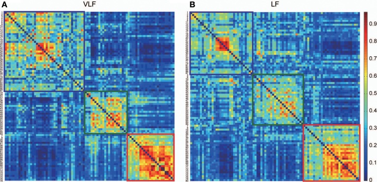
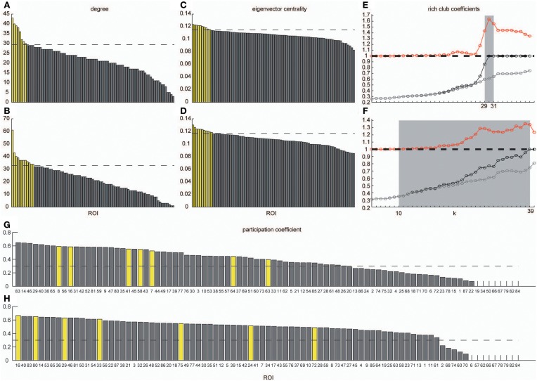
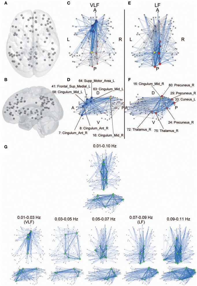
A community is a set of nodes with dense inter-connections, while there are sparse connections between different communities. A hub is a highly connected node with high centrality. It has been shown that both "communities" and "hubs" exist simultaneously in the brain's functional connectivity network (FCN), as estimated by correlations among low-frequency spontaneous fluctuations in functional magnetic resonance imaging (fMRI) signal changes (0.01-0.10 Hz). This indicates that the brain has a spatial organization that promotes both segregation and integration of information. Here, we demonstrate that frequency-specific network topologies that characterize segregation and integration also exist within this frequency range. In investigating the coherence spectrum among 87 brain regions, we found that two frequency bands, 0.01-0.03 Hz (very low frequency [VLF] band) and 0.07-0.09 Hz (low frequency [LF] band), mainly contributed to functional connectivity. Comparing graph theoretical indices for the VLF and LF bands revealed that the network in the former had a higher capacity for information segregation between identified communities than the latter. Hubs in the VLF band were mainly located within the anterior cingulate cortices, whereas those in the LF band were located in the posterior cingulate cortices and thalamus. Thus, depending on the timescale of brain activity, at least two distinct network topologies contributed to information segregation and integration. This suggests that the brain intrinsically has timescale-dependent functional organizations.

Keywords: community; frequency-dependency; functional connectivity; integration; network analysis; resting-state fMRI; rich-club connectivity; segregation.

Figure 1

Procedure for detecting frequency specificity of functional connectivity. Coherence was estimated in all pairs of ROIs between 0.01 and 0.25 Hz, and averaged within narrow, 50%-overlapping frequency bands that had a band width of 0.02 Hz. As a result, we obtained coherence matrices from 23 frequency bands (A). (B) Considering that frequency specificity is different between ROIs in the same functional system and ROIs of two distinct functional systems, coherence values were divided into two categories: coherence values within the same functional system (intra-system), and coherence values between different functional systems (inter-system). The colored parts of the matrix in (B) correspond to the coherence values of the intra-system (black) and inter-system (red). To investigate frequency specificity in these categories, the coherence values were further averaged within each category in each coherence matrix.

Figure 2

Frequency-specificity of functional connectivity. Averaged coherence values in two categories are shown. Black curves represent coherence values averaged within three functional systems and red curves indicate values calculated in the inter-system groups (Figure 1). Error bars show the standard errors. The x-axis represents the center frequencies of the frequency bands, where coherence values were averaged. For all curves, coherence within 0.01–0.03 Hz (very low frequency, [VLF]) and 0.07–0.09 Hz (low frequency, [LF]) were higher than those of other frequency bands.

Figure 3

Coherence spectrum estimated using simultaneously obtained NIRS data. (A) We obtained NIRS signals at 14 cortical regions indicated as blue rings. Cyan dots represent standard reference points used in locating channels of electroencephalography on the scalp. In a previous study, we identified 14 cortical regions, where NIRS signals were obtained, in MNI space to determine ROIs corresponding to each NIRS measurement region for each individual. For detailed methods for the identification and MNI coordinates, please refer to Sasai et al. (2012). As a result, we found one cortical region (medial prefrontal cortex [mPFC]) included in the default mode system (red filled circle) and two bilateral cortical regions (left and right anterior prefrontal cortices [laPFC and raPFC]) contained in the fronto-parietal system (blue filled circles). (B) Voxels corresponding to measured regions by NIRS are shown. Colors are the same as those defined in (A). (C) We calculated the coherence between laPFC and raPFC to investigate the intra-system coherence spectrum (fronto-parietal system), and also estimated the coherence between mPFC and laPFC, and between mPFC and raPFC, to examine the inter-system coherence spectrum (default-mode and fronto-parietal systems). A black line indicates an intra-system pair of ROIs, whereas cyan lines represent inter-system pairs. (D,E) Coherence spectrums of two NIRS signals (oxygenated [oxy-] hemoglobin and deoxygenated [deoxy-] hemoglobin) with two clear peaks corresponding to typical frequency bands of respiratory fluctuation around 0.3 Hz and cardiac pulsations around 1 Hz. High coherences in VLF and LF could still be observed in the spectrum, supporting the idea that higher coherences in these bands are not due to aliasing. (F) Coherence spectrum obtained using fMRI signals extracted from ROIs corresponding to NIRS measurement regions (as shown in B). We confirmed the high coherence values in VLF and LF in this spectrum, supporting the notion that characteristics of the coherence spectrum cannot be attributed to differences in ROI locations between our current and previous studies.

Figure 4

Graph metrics. We calculated the following two graph metrics in two frequency-specific networks (VLF and LF) estimated in each individual data set: (A) modularity, and (B) global efficiency. Blue bars represent the mean of each graph metric obtained, which was computed in networks estimated in the VLF. Red bars indicate the mean graph metric in the LF. In the current study, we selected sparsity of the brain networks (number of existing edges over the maximum possible number of edges) as threshold measurements. Because different threshold values might affect these graph metrics, we examined the between-group differences in these parameters over a wide range of threshold levels (0.05–0.25). Asterisks indicate statistically significant differences between the metrics obtained in the VLFN and the LFN, tested by two-sampled t-tests (p < 0.05, false discovery rate-corrected).

Figure 5

Consistency of community detection between VLF and LF. (A,B) Show consistent assignment matrices Ca obtained in the VLF (A) and LF (B). To emphasize the modular structures, both Ca were reordered by putting the ROIs in the same module next to each other. Detecting communities in both matrices revealed three in the VLF and LF, indicated by squares. The color of each square corresponds to the assigned community detected in each frequency band: blue denotes community 1, green community 2, and red community 3.

Figure 6

Degrees, eigenvector centrality, rich-club coefficients and participation coefficients. Degrees and eigenvector centralities of all nodes were calculated in the group-level network estimated in the VLF and LF. (A) Shows the distribution of degree estimated in the VLF, and (B) shows the distribution of degree estimated in the LF. (C) Corresponds to the distribution of eigenvector centrality estimated in the VLF, and (D) corresponds to the distribution of eigenvector centrality estimated in the LF. Dashed lines express the mean plus one standard deviation. Yellow bars represent nodal metrics above the threshold (the mean plus one standard deviation), and gray bars indicate those below the threshold. We also calculated rich-club coefficients in group-level frequency-specific networks (see “Rich-club detection”). Black curves correspond to Φ(k), gray curves correspond to Φ_meanrand(k), and red curves correspond to Φ_normalized(k). In both (E,F), there is a tendency for Φ(k) to increase with k at a higher rate than Φ_meanrand(k). Ranges of k, where Φ(k) became significantly higher than Φ_meanrand(k), are highlighted by a gray background. (G,H) Show the participation coefficients of all ROIs in the VLF and LF, respectively. Yellow bars represent the coefficients of hubs in each frequency band. Broken lines indicate 0.3, which is the boundary between provincial and connector hubs (see Materials and Methods).

Figure 7

Anatomical perspective of hub regions. (A,B) Eighty-seven ROIs used in the current study are displayed on a surface rendering of the brain using MATcro software distributed by http://www.mccauslandcenter.sc.edu/CRNL/tools/surface-rendering-with-matlab. Hub regions in frequency-specific networks were the seven highest degree nodes in each frequency band (C–F). The yellow node is a hub that is consistently identified in both the VLF (C,D) and the LF (E,F). The blue nodes are hubs identified only in the VLF, and the red nodes are those identified only in the LF. Hubs are represented by large spheres. Blue lines indicate functional connectivity with hubs within the frequency band, and gray lines represent functional connectivity with hubs within the other band. When k = 30 for A^g_VLF and k = 30 for A^g_LF is selected, rich-club organizations are formed with hub regions. Bold lines indicate connections among rich-club nodes, showing dense interconnections. The numbers correspond to those in Table 1. Anatomical labels were selected using AAL. The abbreviations represent the direction in the brain: A, anterior; P, posterior; L, left; R, right; D, dorsal; V, ventral. (G) Hub regions identified within one wide frequency band (0.01–0.10 Hz) and five narrow frequency bands (0.01–0.03 [VLF], 0.03–0.05, 0.05–0.07, 0.07–0.09 [LF], and 0.09–0.11 Hz). All hub nodes are represented with large green colored spheres. The attributes of the lines are the same as described above.

References

1. Aalkjaer C., Boedtkjer D., Matchkov V. (2011). Vasomotion—what is currently thought? Acta Physiol. (Oxf.) 202, 253–269. 10.1111/j.1748-1716.2011.02320.x - DOI - PubMed
1. Achard S., Bullmore E. (2007). Efficiency and cost of economical brain functional networks. PLoS Comput. Biol. 3:e17. 10.1371/journal.pcbi.0030017 - DOI - PMC - PubMed
1. Achard S., Salvador R., Whitcher B., Suckling J., Bullmore E. (2006). A resilient, low-frequency, small-world human brain functional network with highly connected association cortical hubs. J. Neurosci. 26, 63–72. 10.1523/JNEUROSCI.3874-05.2006 - DOI - PMC - PubMed
1. Anderson J. S., Druzgal T. J., Lopez-Larson M., Jeong E. K., Desai K., Yurgelun-Todd D. (2011). Network anticorrelations, global regression, and phase-shifted soft tissue correction. Hum. Brain Mapp. 32, 919–934. 10.1002/hbm.21079 - DOI - PMC - PubMed
1. Baria A. T., Baliki M. N., Parrish T., Apkarian A. V. (2011). Anatomical and functional assemblies of brain BOLD oscillations. J. Neurosci. 31, 7910–7919. 10.1523/JNEUROSCI.1296-11.2011 - DOI - PMC - PubMed