Learning modifies odor mixture processing to improve detection of relevant components

Abstract

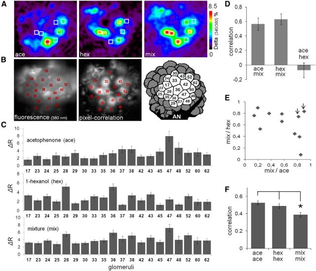
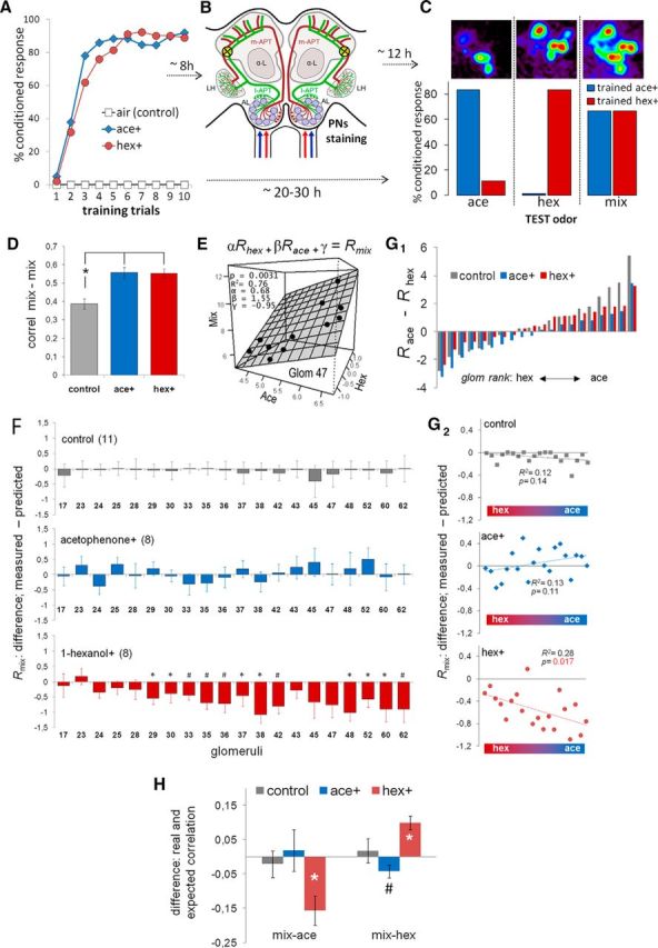
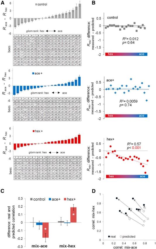
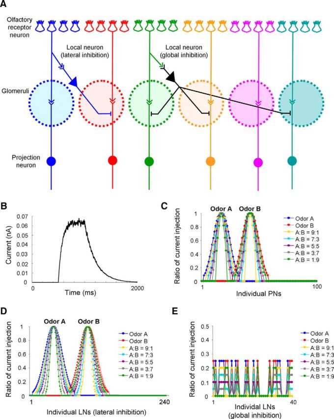
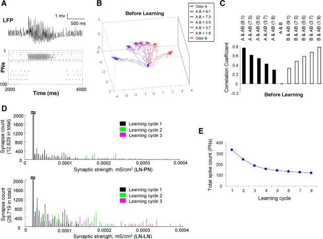
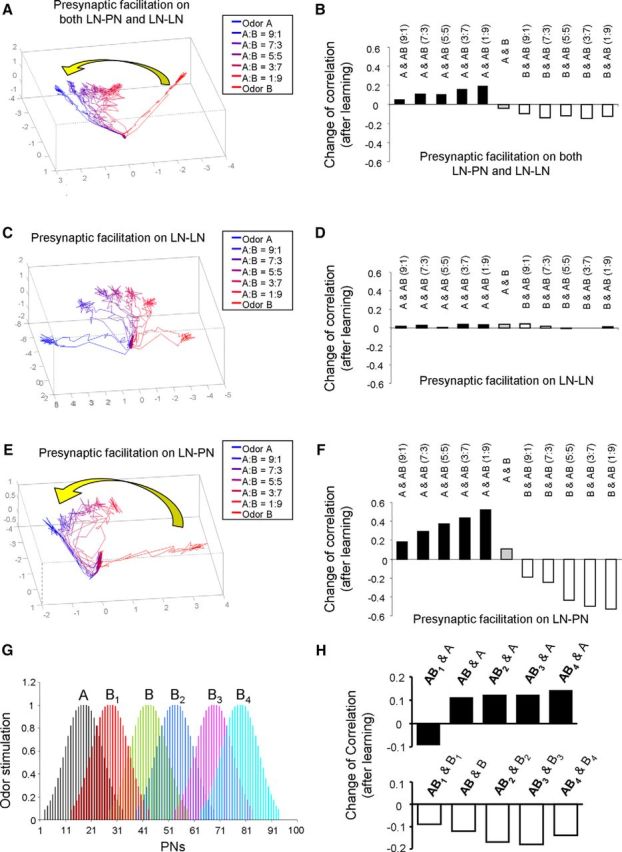
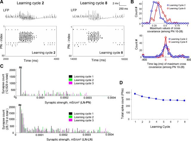
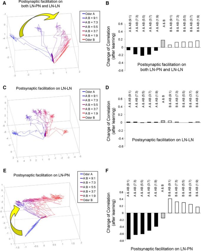
Honey bees have a rich repertoire of olfactory learning behaviors, and they therefore are an excellent model to study plasticity in olfactory circuits. Recent behavioral, physiological, and molecular evidence suggested that the antennal lobe, the first relay of the olfactory system in insects and analog to the olfactory bulb in vertebrates, is involved in associative and nonassociative olfactory learning. Here we use calcium imaging to reveal how responses across antennal lobe projection neurons change after association of an input odor with appetitive reinforcement. After appetitive conditioning to 1-hexanol, the representation of an odor mixture containing 1-hexanol becomes more similar to this odor and less similar to the background odor acetophenone. We then apply computational modeling to investigate how changes in synaptic connectivity can account for the observed plasticity. Our study suggests that experience-dependent modulation of inhibitory interactions in the antennal lobe aids perception of salient odor components mixed with behaviorally irrelevant background odors.

Keywords: antennal lobe; honey bees; olfaction; olfactory learning.

Figure 1.

Imaging of odor elicited calcium signals in projection neurons. A, Color-coded calcium images represent the average of odor responses from 250 to 750 ms after odor onset. From left to right, Images are responses to acetophenone, 1-hexanol, and their mixture (10:10) in the same honey bee. The seven squares represent the same seven glomeruli in different odor responses to aid visualization of the differences between patterns. B, Left, Basal fluorescence image observed with 380 nm excitation light and LP510 emission filter after staining the PNs with FURA-dextran. The glomeruli were identified according to size, shape, and position by comparison with the honey bee AL atlas (Flanagan and Mercer, 1989; Galizia et al., 1999). Middle, Pixel-correlation image (see Materials and Methods) used as an additional tool to aid glomeruli identification. Dark glomeruli do not mean lack of staining; these glomeruli were not activated by the odors and consequently produce low correlation values between neighboring pixels. Right, Schema of the dorsal view of the AL showing the 20 glomeruli used in our analyses. AN, Antennal nerve. C, Quantitative evaluation of the odor responses via change of fluorescence from the reference window (ΔR) from 250 to 750 ms after odor onset in 20 glomeruli. Average ± SEM of odor responses from 11 control bees (top to down: acetophenone, 1-hexanol, and mixture). Numbers in the abscissa correspond to the identity of the glomeruli. D, Pearson's correlation coefficients between response patterns were used to evaluate similarity between odor patterns. The correlation coefficients of three different pairs (ace-mix, hex-mix, ace-hex) were calculated in each control bee. Data are average ± SEM of 11 control bees. E, Scatter plot of the correlation coefficients between mixture and either pure components (hexanol or acetophenone). Each point represents one control bee. Two arrowheads indicate two bees with the highest correlation coefficients between the pure components. F, Correlation coefficients between patterns elicited by the same odor in different bees. Vertical bars represent average ± SEM from a total 55 correlation values that result from arranging 11 controls bees in pairs. The representation of mixture was less conserved across animals than the representation of the pure odors. *p < 0.01 contrasts after ANOVA (F_(2,162) = 6 0.97; p = 0.001).

Figure 2.

Changes in the responses to the mixture after appetitive olfactory conditioning. A, Three groups of bees were trained using appetitive conditioning. Each bee received 10 trials with 2 m sucrose solution separated by 10 min intertrial intervals. Control bees received the reward paired with clean air provided by the odorgun. The other two groups received 1-hexanol or acetophenone as conditioned odor. Learning performance was recorded during conditioning as percentage of animals that extended the proboscis upon stimulation with odor. B, Eight hours after conditioning, projection neurons were stained bilaterally using fura-dextran targeted to where the l-APT enters the lateral calyces of the mushroom bodies (yellow circles). m-APT, Medial antenno-protocerebal tract; l-APT, lateral antenno-protocerebral tract; LH, lateral horn; α-L, alpha lobe. C, On the next day, the bees were prepared for calcium imaging of odor-induced signals on the dorsal side of the antennal lobe (top). Activity patterns were measured three times each to 1-hexanol, acetophenone, and the binary mixture, presented in random order separated by 1 min intervals. A set of trained bees not stained for imaging was used to determine the strength of olfactory memory and odor discrimination (bottom). All honey bees underwent three test trials without reward using: (1) the conditioned odor (1-hexanol or acetophenone), (2) a different odor that they have not experienced before (1-hexanol or acetophenone), and (3) the binary mixture containing both odors in same proportion. Bar colors represent the odor used for conditioning. The order of the three odors was randomized across animals (1-hexanol-trained bees, n = 20; acetophenone-trained bees, n = 18). Control bees are not shown because they did not evoke any conditioned response. D, Average ± SEM of the correlation coefficients between mixture-elicited activation patterns across bees. The correlation was calculated between bees from the same training group: control (gray), ace⁺ (blue), and hex⁺ (red), ANOVA: F_(2,108) < 0.0001. *p < 0.001 (post hoc contrasts). E, A best fit linear equation was obtained for each glomerulus to estimate the response of the mixture as a function of the responses to 1-hexanol and acetophenone. Graph represents an example of the best-fit linear equation (plane) of glomerulus 47 derived from 11 data points (11 control bees). F, Average ± SEM of the difference between the measured and the predicted response to the mixture for each glomerulus in the three different groups of bees. The numbers in the abscissa indicate the identification of the glomeruli. The differences shown in the graph were calculated as the measured response minus the predicted response. *p < 0.05, between measured and predicted values (paired t test). ^#p < 0.01, between measured and predicted values (paired t test). From top down, control group (n = 11), ace⁺ group (n = 8), and hex⁺ group (n = 8). G₁, Glomeruli were ranked according to the difference of the average response to 1-hexanol and acetophenone in control bees. The ranking was made by subtracting the response to 1-hexanol (R_hex) from the response to acetophenone (R_ace). G₂, The points in these plots correspond to the data (R_mix: measured − predicted) shown in F, but reorganized along the abscissa according to the ranking derived from G₁. The red/blue color bar at the bottom of each plot represents the ranking of glomeruli from hexanol responders to acetophenone responders. The results of a linear regression analysis are displayed in each plot. H, The predicted responses to the mixture for each glomerulus were arranged to establish a predicted response pattern to the mixture. The correlation between patterns elicited by the pure odors and the predicted pattern to the mixture were designated predicted correlations. The figure shows the average ± SEM of the differences between the real and the predicted correlation between responses to the mixture and responses to the pure odors (mix-ace, mix-hex) in the three groups of bees (control, ace⁺, hex⁺). *p < 0.001, between real and predicted correlation (paired t test). ^#p = 0.06, in the case of correlation mix-hex after conditioning with acetophenone.

Figure 3.

Changes of correlation between the responses to the mixture and the pure odors based on individual bee response profiles. A, Glomeruli were ranked according to the difference of response to acetophenone and 1-hexanol in each individual bee. Three groups of bees (from top down: 11 control bees; 8 ace⁺ bees; 8 hex⁺ bees) are shown. In the tables: each row represents one bee, each column represents one category, and the numbers in the table indicate the identity of the glomeruli. The graphs (bars) show the average ± SEM of the difference between the responses to acetophenone and 1-hexanol in each group of bees along the ranking category (1–20). B, For each group of bees, the average of the difference between measured and predicted response to the mixture was plotted along the ranked categories (1–20). C, The average ± SEM of the differences between real and predicted correlation coefficients between the mixture and either pure components were calculated in each group of bees. *p < 0.001 (paired t test). D, For hex⁺ group, a scatter plot showing the predicted and real correlation coefficient between the mixture and the pure components. The eight open circles represent predicted correlation coefficients of eight bees in the hex⁺ group; the eight filled circles represent the real correlation coefficient in the same eight bees. The arrows indicate the shift from the predicted correlation to the real correlation of the same bee.

Figure 4.

Settings of AL network model and odor stimulation. A, Structure of the AL network model (for details, see Table 1). B, The temporal pattern of full current injection (ratio = 1) in each stimulation cycle (2 s). C, The spatial patterns of odor stimuli (current injections), including odor A, odor B, and their binary mixtures (A:B = 9:1, 7:3, 5:5, 3:7, 1:9) to 100 PNs. D, The spatial patterns of current injection across 240 LNs (lateral inhibition). E, The spatial patterns of current injection across 40 LNs (global inhibition).

Figure 5.

Olfactory responses in AL before learning and after learning modified by presynaptic facilitation. A, Before learning, the LFP in AL and the rastergram across whole population of PNs in responding to odor A are displayed. B, Before learning, spatiotemporal patterns of two pure odor and five mixture odor responses across all PNs are displayed in a PCA space. A smooth transition of trajectories along mixture ratios is observed. C, Before learning, the correlation coefficients between two pure odors and between pure odor and mixture odors are shown. D, During learning of odor A, the synaptic strength of LN-PN and LN-LN was facilitated based on presynaptic spiking activities in LN. These two histogram plots show distribution of synaptic weights of 12,629 LN-PN synapses (top) and 28,719 LN-LN synapses (bottom) during the first three learning cycles indicated by different colors. E, Total PNs' spike count dropped mainly during the first few learning cycles.

Figure 6.

Changes of odor responses in AL after learning based on presynaptic facilitation. A, After learning of odor A manipulated by presynaptic facilitation in both LN-PN and LN-LN synapses, the dynamic trajectories of odor responses based on activities across all PNs are presented in 3D PCA space. The trajectories of mixtures were found to shift closer to the trajectory of learned odor, odor A. B, Corresponding to A, the change of correlation coefficient derived before and after olfactory learning was also calculated. It was found that, after learning of odor A, the correlation coefficient between odor A and mixture odors increased. On the other hand, the correlation coefficient between odor B and mixture odors reduced. C, In the second setting, the presynaptic facilitation mechanism was installed in LN-LN synapses only. In PCA space, the trajectories of mixture odors stay at the middle between the trajectories of odor A and odor B after learning without obvious shift toward either pure odor component. D, Corresponding to C, the change of correlation coefficient between odor responses was quite small after learning. E, In the third setting, the presynaptic facilitation mechanism was installed in LN-PN synapses only. The trajectories of mixture odors in PCA space were found to move toward the learned odor, odor A. F, Corresponding to E, the correlation coefficients between odor A and mixture odors were increased significantly after learning. On the other hand, the correlation coefficients between odor B and mixture odors were decreased. G, The spatial patterns of alterative odor B (including B₁, B₂, B₃, and B₄) were plotted. These alternative odors were also used to test the impact of presynaptic facilitation on olfactory responses. H, Following G, the degree of similarity between pure odor and mixture odor (5:5) responses was evaluated by correlation coefficients across PNs. Top, The correlation between mixture odors and odor A increased after learning of odor A, except one of the mixture odors, AB₁. Bottom, The correlations between all mixture odors and odor B reduced after learning of odor A.

Figure 7.

Results of olfactory learning manipulated by postsynaptic facilitation. A, As the postsynaptic facilitation mechanism was effective in both LN-PN and LN-LN, the trace of LFP and the rastergram of all PNs obtained from learning cycle 2 (left panel) and cycle 8 (right panel) are exhibited. It was noticed that, after experiencing several learning cycles, the firing activities became more synchronous across PNs (comparing cycle 8 with cycle 2 here). B, Corresponding to A, the level of synchronization across active PNs (PN 10-PN 28) was further evaluated by cross-covariance analysis. After several cycles of learning, the PNs' firing patterns became more synchronous indicated by larger values of maximum cross-covariance (top, red distribution) and overall shorter time lag to the main peak (bottom, red distribution). C, Changes of synaptic strength distribution during the first three cycles of learning of odor A in the model with postsynaptic facilitation in LN-PN and LN-LN. D, The total spike number in PNs along learning cycles modified by postsynaptic facilitation in LN-PN and LN-LN. Decrease of total spike number (mostly the first 3 or 4 cycles) was observed.

Figure 8.

Changes of odor responses after learning manipulated by postsynaptic facilitation. A, After learning of odor A via manipulation of postsynaptic facilitation in both LN-PN and LN-LN, the trajectories of mixture odor responses moved toward the unlearned odor, odor B, in PCA space. B, Corresponding to A, after learning of odor A, the correlation coefficient between odor A and mixture odors reduced. On the other hand, the correlation coefficient between odor B and mixture odors increased. C, After learning of odor A manipulated by postsynaptic facilitation in LN-LN synapses only, the mixture odors stayed at middle between odor A and odor B in PCA space. D, Corresponding to C, the changes of correlation coefficient among odor responses are small. E, When postsynaptic facilitation was set up at LN-PN synapses only, the trajectories of mixture odors were found to move toward the unlearned odor, odor B. F, Corresponding to E, the correlation coefficients between odor A and mixture odors reduced. At the same time, the correlation coefficients between odor B and mixture odors increased.

References

1. Antonov I, Antonova I, Kandel ER, Hawkins RD. Activity-dependent presynaptic facilitation and hebbian LTP are both required and interact during classical conditioning in Aplysia. Neuron. 2003;37:135–147. doi: 10.1016/S0896-6273(02)01129-7. - DOI - PubMed
1. Aso Y, Siwanowicz I, Bräcker L, Ito K, Kitamoto T, Tanimoto H. Specific dopaminergic neurons for the formation of labile aversive memory. Curr Biol. 2010;20:1445–1451. doi: 10.1016/j.cub.2010.06.048. - DOI - PMC - PubMed
1. Assisi C, Stopfer M, Laurent G, Bazhenov M. Adaptive regulation of sparseness by feedforward inhibition. Nat Neurosci. 2007;10:1176–1184. doi: 10.1038/nn1947. - DOI - PMC - PubMed
1. Bazhenov M, Stopfer M, Rabinovich M, Abarbanel HD, Sejnowski TJ, Laurent G. Model of cellular and network mechanisms for odor-evoked temporal patterning in the locust antennal lobe. Neuron. 2001a;30:569–581. doi: 10.1016/S0896-6273(01)00286-0. - DOI - PMC - PubMed
1. Bazhenov M, Stopfer M, Rabinovich M, Huerta R, Abarbanel HD, Sejnowski TJ, Laurent G. Model of transient oscillatory synchronization in the locust antennal lobe. Neuron. 2001b;30:553–567. doi: 10.1016/S0896-6273(01)00284-7. - DOI - PMC - PubMed
Publication types
LinkOut - more resources