Biogeographic patterns of bacterial microdiversity in Arctic deep-sea sediments (HAUSGARTEN, Fram Strait)

Abstract

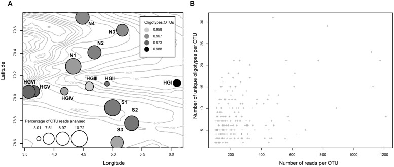
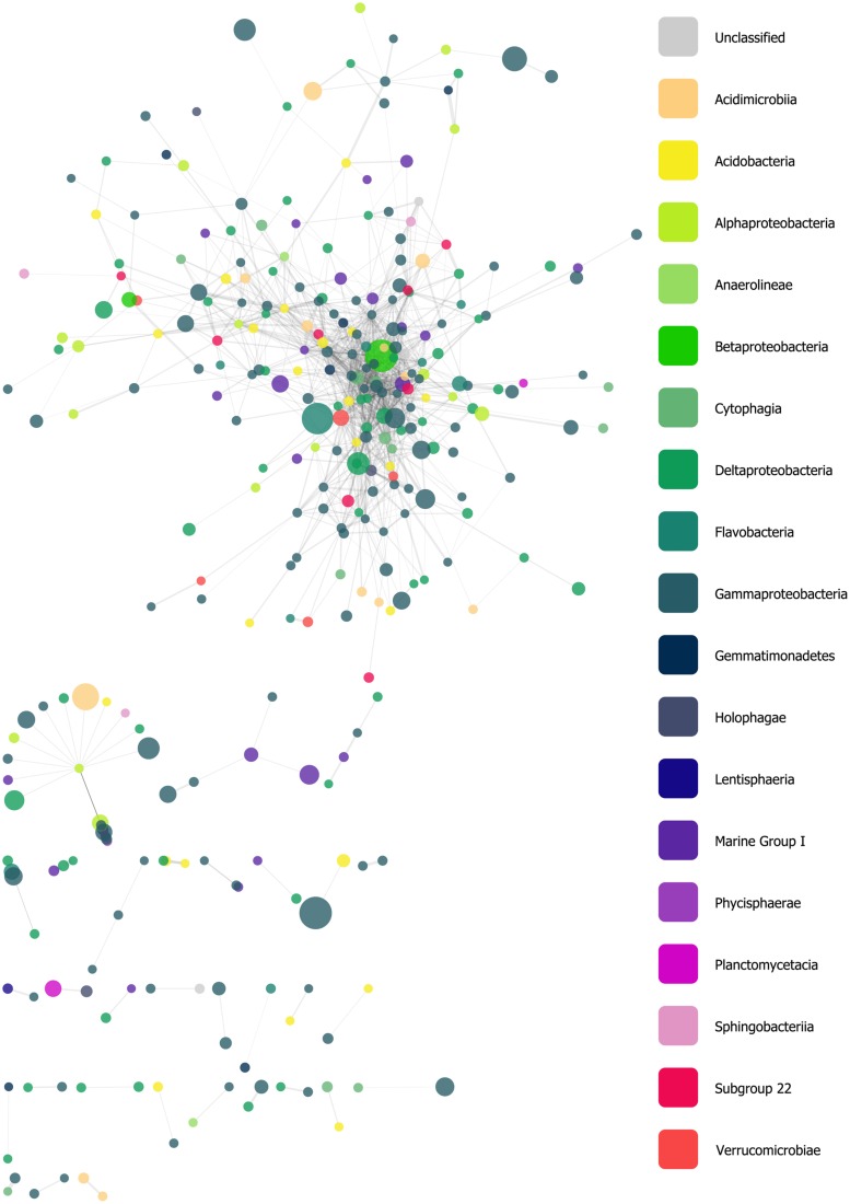
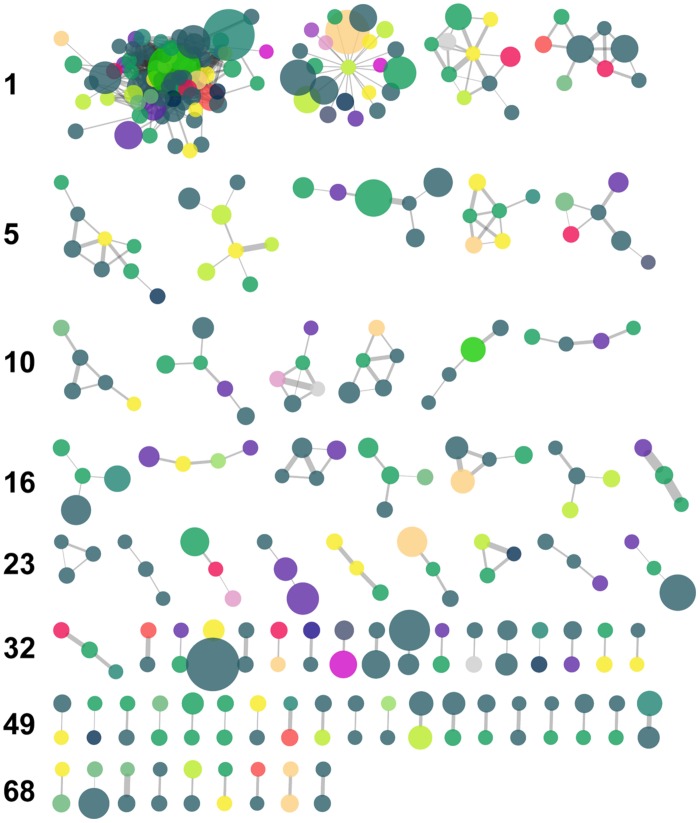
Marine bacteria colonizing deep-sea sediments beneath the Arctic ocean, a rapidly changing ecosystem, have been shown to exhibit significant biogeographic patterns along transects spanning tens of kilometers and across water depths of several thousand meters (Jacob et al., 2013). Jacob et al. (2013) adopted what has become a classical view of microbial diversity - based on operational taxonomic units clustered at the 97% sequence identity level of the 16S rRNA gene - and observed a very large microbial community replacement at the HAUSGARTEN Long Term Ecological Research station (Eastern Fram Strait). Here, we revisited these data using the oligotyping approach and aimed to obtain new insight into ecological and biogeographic patterns associated with bacterial microdiversity in marine sediments. We also assessed the level of concordance of these insights with previously obtained results. Variation in oligotype dispersal range, relative abundance, co-occurrence, and taxonomic identity were related to environmental parameters such as water depth, biomass, and sedimentary pigment concentration. This study assesses ecological implications of the new microdiversity-based technique using a well-characterized dataset of high relevance for global change biology.

Keywords: Arctic LTER; HAUSGARTEN; deep sea sediments; oligotyping; taxonomic resolution.

FIGURE 1

(A) Bubble plot approximating the location of each sampling site (bubble coordinates), the per site, percentage contribution of reads used in this study (bubble size), and the sample-specific ratio of the number of reads that were present in an oligotype to the number of reads in the OTU it was derived from (fill intensity). Numeric values on isobaths indicate the depth of the seafloor in meters below the water surface. (B) The total number of reads clustered in a given OTU plotted against the number of oligotypes derived from that OTU (Pearson’s R² = 0.39, P <<0.01).

FIGURE 2

The oligotype:OTU ratio for each (A) Phylum (B) Class and (C) Order analyzed.

FIGURE 3

Heatmaps illustrating examples of abundance matrices subject to checkerboard and togetherness score screening. Rows (oligotypes) have been Hellinger transformed and ordered by hierarchical cluster analysis using average linkage and Bray–Curtis dissimilarities. Darker shades indicate higher relative abundance of reads. In the following text, the maximum, untransformed number of oligotype reads in each OTU-derived relative abundance matrix is noted in brackets. The oligotypes for OTUs (A) EUGQ5 [8], which had the joint-highest average T score observed; (B) B177D [5], which had both the highest average C and T scores observed; (C) C60MC [12]; and (D) DON2B [9] which both had high average C and T scores are displayed (cf. Table 2). AGCT: nucleotides; -: gap.

FIGURE 4

Heatmaps and RDA triplots (type 2 scaling) derived from Hellinger-standardized, OTU-specific oligotype relative abundance matrices. The seven models shown had at least 50% constrained variance and were significant at a P-value threshold of 0.05 (FDR-corrected) cf. Table 3. The depth and latitudinal gradients sampled are reflected in the sample order (HGI shallowest, HGVI deepest, N4 northernmost, S3 southernmost) and elaborated upon in the bottom right of the figure where the depth and latitudinal gradients are highlighted with red and blue boxes, respectively. Site HGIV, the central site of the intersecting transects, belongs to both transects. See Figure 1A Jacob et al. (2013) for greater detail. When other explanatory variables were featured in the model, an additional heatmap of these variables’ z-scored values is included in the panel. Across heatmaps, darker shades indicate higher, Hellinger-transformed relative abundance of reads or higher values of a given explanatory variable. The panels reference oligotype abundance matrices derived from the following OTUs (the maximum, untransformed read abundance across oligotypes in each matrix is noted in brackets): (A) BJCLU [18] (B) AV4R2 [14] (C) BGP4M [16] (D) D3V9F [62] (E) DTNEI [19] (F) AHWYC [39] and (G) ANOZB [9]. Explanatory variables are represented by gray text and arrows pointing in their direction of increase, these comprise Porosity (range: 51.8–72.3% volume), CPE (18.86–44.26 μg cm^-3), Northing (8727035–8850377 m), Easting (512100–565125 m), and Depth (1284–3535 m). Oligotypes (response variables) are ordinated as bold, red text. Relative to each plot’s origin, the position of an oligotype’s ordination indicates its direction of increase. Angles between variables indicate their linear correlation, with an angle of 0° indicating perfect positive correlation, 180° indicating perfect negative correlation, and 90° indicating orthogonality. Samples are ordinated as black text. Transparency effects are used to improve visibility in congested regions of the triplots and have no meaning.

FIGURE 5

Force-directed, spring-embedded network displaying oligotypes (nodes) with Whittaker’s index of association (IA) values greater than 85 (FDR-corrected P-values as determined by 200 permutations <0.05), represented as edges. Nodes are color-coded by taxonomic Class. See text for a summary of this network’s general statistics.

FIGURE 6

Results of Markov clustering of the graph displayed in Figure 5, with a granularity parameter value of 2.5. Nodes are color-coded by taxonomic Class (see Figure 5 for key) and their size is proportional to the total relative abundance of the corresponding oligotype. Edge thickness is proportional to the value of the IA between oligotypes. The leftmost cluster of each row is numbered along the left margin.

References

1. Bauerfeind E., Nöthig E. M., Beszczynska A., Fahl K., Kaleschke L., Kreker K., et al. (2009). Particle sedimentation patterns in the eastern Fram Strait during 2000–2005: results from the Arctic long-term observatory HAUSGARTEN. Deep Sea Res. Part 1 Oceanogr. Res. Pap. 56 1471–1487 10.1016/j.dsr.2009.04.011 - DOI
1. Benjamini Y., Hochberg Y. (1995). Controlling the false discovery rate: a practical and powerful approach to multiple testing. J. R. Stat. Soc. Ser. B Stat. Methodol. 57 289–300 10.2307/2346101 - DOI
1. Bienhold C., Boetius A., Ramette A. (2012). The energy-diversity relationship of complex bacterial communities in Arctic deep-sea sediments. ISME J. 6 724–732 10.1038/ismej.2011.140 - DOI - PMC - PubMed
1. Bivand R., Keitt T., Rowlingson B. (2013). rgdal: Bindings for the Geospatial Data Abstraction Library. R Package Version 0. 8–11 Available at: http://CRAN.R-project.org/package=rgdal
1. Blanchet F. G., Legendre P., Borcard D. (2008). Forward selection of explanatory variables. Ecology 89 2623–2632 10.1890/07-0986.1 - DOI - PubMed
LinkOut - more resources