Synaptic consolidation: from synapses to behavioral modeling

Abstract

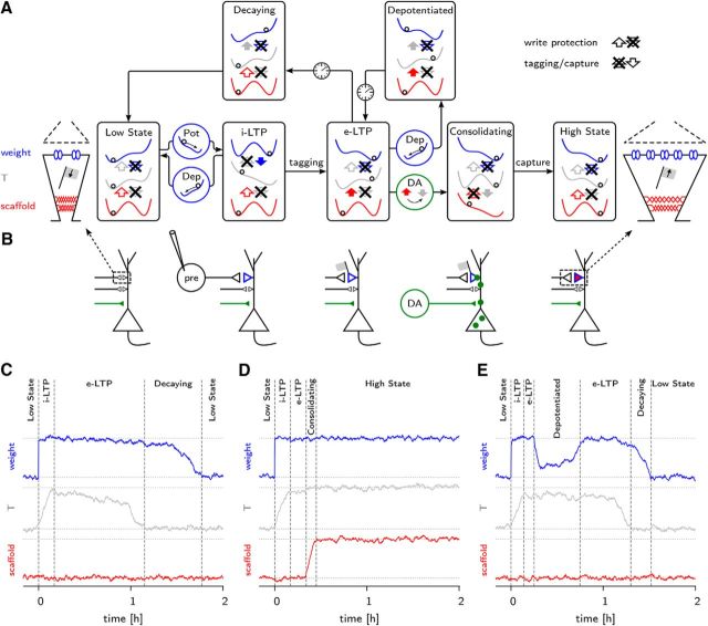
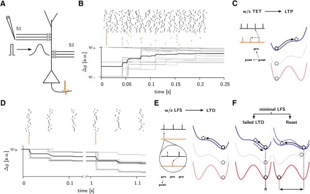
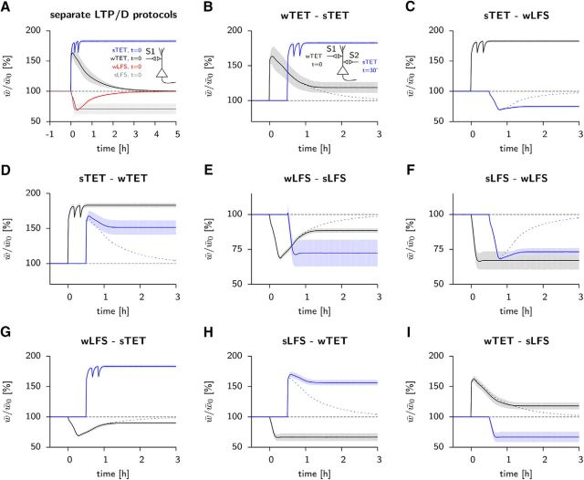
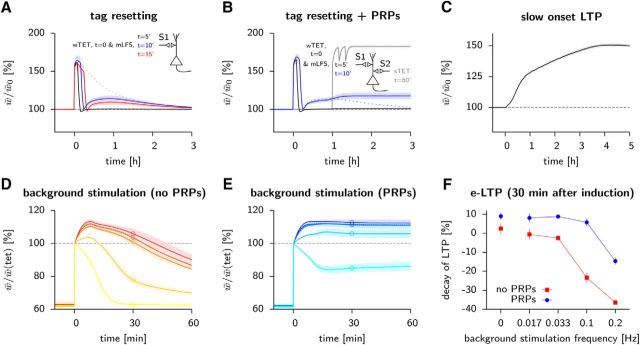
Synaptic plasticity, a key process for memory formation, manifests itself across different time scales ranging from a few seconds for plasticity induction up to hours or even years for consolidation and memory retention. We developed a three-layered model of synaptic consolidation that accounts for data across a large range of experimental conditions. Consolidation occurs in the model through the interaction of the synaptic efficacy with a scaffolding variable by a read-write process mediated by a tagging-related variable. Plasticity-inducing stimuli modify the efficacy, but the state of tag and scaffold can only change if a write protection mechanism is overcome. Our model makes a link from depotentiation protocols in vitro to behavioral results regarding the influence of novelty on inhibitory avoidance memory in rats.

Keywords: consolidation; modeling; synaptic tagging.

Figure 1.

States and transitions of the synapse model. Potentiating protocols applied to the model have different outcomes. A, Schematic view of the different synaptic states. On the left is a sketch of the low state of a synapse. It consists of three elements, a weak weight (blue) and two hidden variables, the tagging-related variable T (gray), currently in its lower state, and a small scaffold (red). The diagram focuses on potentiation from the low to the high state. The synapse's internal variables are represented by three double well potentials (blue, gray and red curves). These variables are coupled to each other (shown by large arrows), which alters their stability properties. A variable in its low state is represented by a ball on the left side of a panel and a variable in its high state by a ball on the right side. The directions of the couplings depend on the synapse state and on its recent history. In the low state, all three variables are in the lower potential well and the couplings are upstream, from the scaffold to the tagging variable T and from T to the weight. A potentiating plastic event carries the weight to its strong state (w = +1) without affecting the two other layers. It also reverses the coupling from the weight to T. The synapse exhibits then initial LTP. After LTP induction, within ∼10 min, a tag is set (T = +1) due to the influence of the first layer on the second (filled blue arrow). The coupling between the first two layers then comes back to its resting direction from bottom to top. If an appropriate neuromodulation (e.g., dopamine) is delivered to the postsynaptic neuron, production of PRP is triggered, allowing for stabilization of recent plastic changes. It reverses the direction of the coupling between T and the scaffold for ∼2 h, enabling the last layer to follow its neighbor to the large state (z = +1). This changes the long-term stability of the synapse. In the absence of external input, a tagged synapse decays back to its resting state within a few hours. The timescale of the decay is determined by the time needed for noise to push T out of the metastable potential well. When a depotentiating protocol is applied to a tagged synapse, the weight is reset to its weak state. Both the first and second layer are then in a metastable situation. Because the potential barrier for the weight is lower than for T, the weight will bounce back up, setting the synapse back into the e-LTP state. It allows either for capture of PRPs if there was any dopamine release or for decay to the synapse's low state. This stands in contrast to the case in which depotentiation occurs before a tag had time to be set. In this situation, the synapse is directly set back to the low state. On the right of the diagram is a sketch of the high state of a synapse. In contrast to the sketch on the left, the weight is strong, T is up, and the scaffold is large. B, Sketch of a postsynaptic neuron and of its incoming synapses. The upper synapse's state corresponds to the one in A directly above. A synapse can be in the low state (small black triangle), in the i-LTP state (large blue triangle), in the e-LTP state (blue triangle and gray flag), or in the high state (blue triangle filled in red). Consolidation occurs through the presence of PRPs (green circles). C, Typical behavior of a synapse during an e-LTP-inducing protocol. We show the time course of the three layers of a synapse (blue, gray, and red lines) and the synaptic state to which it corresponds. D, As in C, but with a stronger stimulus-inducing l-LTP. Note that consolidation occurs because of the presence of PRPs. E, As in C, with a resetting stimulus 15 min after the start of potentiation.

Figure 2.

Stimulation protocols. A, Two groups (S1 and S2) of 2000 input units project onto 10 AIF neurons (only one is shown) with a connection probability of 10%. An extracellular stimulation pulse is modeled by a Gaussian packet of action potentials with a SD of 3 ms, with 1 spike per axonal projection. For three or fewer consecutive packets separated by 50 ms (as in a sLFS protocol, see D), a postsynaptic neuron generates a single spike, whereas several spikes are emitted if stimulation occurs at 100 Hz (as in a wTET, see B). B, Detailed view of a wTET protocol. Spike arrivals at 20 synapses (black bars) are shown together with spikes of all 10 postsynaptic units (red bars). The effect on individual weights can be seen in the bottom (gray lines). Note that potentiation happens only after the second postsynaptic spike of a neuron. Only those synapses crossing the long-term stability barrier (dashed horizontal line) will undergo a long-lasting change. The mean weight is shown in black. C, Tetanic stimulation protocols. A wTET (21 pulses at 100 Hz) or a sTET (3 × 100 pulses at 100 Hz) is strong enough to overcome neuronal adaptation so that the postsynaptic neuron fires several spikes (red bars, schematic). Because potentiation needs at least two postsynaptic spikes (post-pre-post triplet), a high postsynaptic firing rate gives rise to LTP (Pfister and Gerstner, 2006; Clopath et al., 2010), indicated as a shift to the metastable state on the right. D, With a sLFS protocol (3 pulses at 20 Hz repeated every second), the postsynaptic neuron fires only once per second (top, interrupted time axis). Synapses initially in the high state (gray traces) become weaker on average (black). Note that the first and second volley of spike arrivals, ∼50 ms after the postsynaptic spike, lead to synaptic depression. E, Low-frequency stimulation protocols. During a sLFS, we have one postsynaptic spike (red bar, schematic) for three presynaptic spikes (black) at the same synapse arising from three subsequent stimulation volleys, which gives rise to a strong post-before-pre LTD. During a wLFS (900 pulses at 1 Hz, top), the postsynaptic neuron fires once per volley, but because spikes arrive approximately in the middle of the packet (compare first stimulus in D), approximately half the synapses perceive a post-before-pre pattern leading to LTD, whereas the other half perceives an isolated pre-before-post causing no effect. The accumulation of the 900 pulses makes the LTD stimulus strong enough to have a long-lasting effect. In the case of an sLFS, the larger fraction of post-before-pre spikes gives rise to a larger effect. F, Resetting effect. A reset protocol (250 at 1 Hz) is not enough to produce any LTD on a synapse in the high state (left) because the number of pulses is not enough to push the weight variable over the potential barrier. For a synapse in the e-LTP state (right) the barrier for depression is lower because the meta-stable position of the tag is somewhat shifted to the left. This enables softer protocols to have a clear depotentiation effect.

Figure 3.

The model accounts for classic tagging and cross-tagging experiments. One (A) or two (B–I) groups of 2000 Poisson neurons project onto 10 postsynaptic AIF neurons with 10% connection probability. A, Four standard stimuli used in hippocampal slice tagging experiments simulated separately: a wTET consisting of 21 pulses at 100 Hz (black), a sTET, 3 blocks of 100 pulses at 100 Hz separated by 10 min (blue), a wLFS, 900 pulses at 1 Hz (red) and an sLFS, 900 blocks of 3 pulses at 20 Hz separated by 1 s (gray). Only the two strong stimuli involve delivery of dopamine, necessary for stabilization of the changes. The weak stimuli decay to baseline within a few hours. The evolution of the mean scaled synaptic weight w̄/w̄₀ is shown (lines) together with its SD over 10 repetitions (shaded area). B, e-LTP is rescued by a strong stimulus. Thirty minutes after a wTET has been applied on a first pathway (S1, black), another set of synapses onto the same neurons (S2, blue) experience a sTET, making PRPs available to all synapses. The dashed line represents a weakly tetanized pathway in a different neuron for comparison. C, Cross tagging between potentiation and depression. A sTET in one pathway (S1, black) can provide the PRPs necessary for the stabilization of synapses after a wLFS applied on another pathway (S2, blue). The time course of a wLFS alone is shown for comparison (dashed line). D–I, Other combinations of weak and strong stimuli in synaptic tagging and capture. Synapses on the first pathway (S1) are shown in black, those on the second pathway (S2) in blue. Dotted lines show the outcome of the weak protocol on a separate slice without interaction. wTET/sTET, Weak/strong tetanic stimulation; wLFS/sLFS, weak/strong low-frequency stimulation.

Figure 4.

Nonstandard synaptic tagging and capture. A, Tag resetting: if a depressing stimulus is applied shortly after a wTET on the same pathway, the synaptic weights are reset to their weak state (w = −1). If the reset happens 5 min after potentiation no tag had time to be set (T = −1) and the mean weight lies on the 100% line (black line). When the time difference is longer than 10 minutes, a rebound can be observed (blue and red lines) due to the synaptic tags dragging along the corresponding weights back to the strong state (T = +1, w → + 1). B, As in A, except PRPs are made available via an sTET on a second pathway (S2) 1 h after the wTET on the first pathway (S1). When the time difference between potentiation and depotentiation is ∼10 min, synapses can experience consolidation (blue line). C, Slow onset LTP. If, every few minutes, a weak stimulus is applied in the presence of dopamine (see Materials and Methods), synaptic weights slowly increase over hours. D, The decay of e-LTP is activity dependent. After an LTP induction protocol (100 pulses at 100 Hz), we randomly stimulated model neurons to fire at some background frequency ranging from 0 Hz (red) to 0.2 Hz (yellow), in the absence of PRP. E, As in D, but in the presence of PRP for the same frequency range (from blue to cyan). F, Amount of decay 30 min after tetanization without (red symbols corresponding to the circles in D; vertical bars are SD over 10 repetitions) or with PRPs available (blue symbols, corresponding to the circles in E). Increasing the frequency accelerates the decay when no consolidation is present due to the resetting effect as the frequency approaches 1 Hz. Up to ≈0.1 Hz, PRPs are able to rescue early changes. Past this limit, the weights are reset before tags are set.

Figure 5.

Behavioral simulation paradigm. A, Network architecture. The input consists of three patterns of ∼500 Poisson neurons each with a 10% overlap and projects to the spatial population and to the action units. The spatial cluster is composed of 1000 excitatory AIF neurons and 250 inhibitory LIF neurons that project to the fear population consisting of 100 LIF neurons that inhibit the 10 × 100 AIF action neurons. Background Poisson input (ext) is given to the spatial cluster and to the fear neurons via one-to-one connections (dashed arrows). Plastic connections (or neuromodulation thereof) are shown in red. B, Rate distribution in the spatial module in the absence (black) and during presentation of a spatial cue (gray). The spike raster shows that a few neurons are highly active after stimulus onset. C, Two-dimensional histogram of the momentary synaptic weights from spatial to fear neurons immediately after IA training. The horizontal axis represents the firing rate of neurons in the spatial module while the simulated rat is in the training cage. The gray value indicates the fraction of synapses with a given presynaptic firing rate (horizontal) and a given weight (vertical axis). Only the highly active spatial neurons have strong links to the fear neurons (top-right corner). Other connections remain weak because the weights stay below the barrier (dashed horizontal line) and therefore eventually decay back to the low state. D, Jump mechanism. The simulations are stopped and the jump time is recorded when the firing rate (averaged over 0.1 s) in the majority of the population encoding the action jump hits a threshold (dashed red line). We show two example traces in a naive scenario (black) and in a situation where fear is present (gray). On the left firing rate distributions show the inhibitory effect of encoded fear. Top, Histograms of jump times in the naive case (black) and in a case where fear is present (gray).

Figure 6.

Behavioral simulations results. A, Latencies during inhibitory avoidance training (white boxes) and at different times t* after training (gray boxes, for t* = 15 min, 60 min, 24 h) in the case of a weak foot shock (paired t tests, n = 10; t* = 15, p < 0.001; t* = 60, p = 0.049). A stronger stimulation involving dopamine delivery (strong) is able to rescue the memory trace (p < 0.001), which otherwise has disappeared after t* = 24 h. Error bars show SD. B, Long-term memory can also be rescued by novelty. If an OF setup was applied to the network either before (−t) or after (+t) the fear encoding in a specific time window, the dopamine delivery associated to it could trigger the necessary protein synthesis to consolidate the synaptic connections (paired t tests, n = 10; t = −120, p = 0.028; t = −60, p < 0.001; t = +15, p = 0.004). The hole at t = +0 is due to a reset of previously formed connections during the OF stimulation. Because it happens within the 10 min window when tags were not set yet, the memory trace is totally erased.

Figure 7.

Synaptic traces during behavioral protocol. A, OF exploration preceding inhibitory avoidance training (OF → IA) by 1 h. Top, Weight traces of three individual synapses (blue lines) from input neurons active in the training cage to neurons in the spatial population. Bottom, Mean weight over all synapses originating from input neurons that are highly active in the training cage. B, As in A but with a delay of 2 h between OF and training. C, OF exploration following inhibitory avoidance training after 30 s. Top, Individual synaptic weight traces. Bottom, Mean synaptic weight. Note the rapid increase and immediate reset of weights. D, As in C but with a time difference of 15 min. During OF exposure, synapses are depotentiated. Whereas one of the sample synaptic weight traces (blue) remains at the low value after the OF stimulation, two others recover to their high values. The result for the mean weight (black line, 113% at t = 15 minutes and 109% at t = 40 minutes) indicates that ∼70% of those synapses that were tagged before OF exposure returned to their high efficacy values thereafter.

References

1. Abraham WC, Bear MF. Metaplasticity: the plasticity of synaptic plasticity. Trends Neurosci. 1996;19:126–130. doi: 10.1016/S0166-2236(96)80018-X. - DOI - PubMed
1. Abraham WC. Metaplasticity: tuning synapses and networks for plasticity. Nat Rev Neurosci. 2008;9:387. doi: 10.1038/nrn2356. - DOI - PubMed
1. Amit D, Fusi S. Learning in neural networks with material synapses. Neural Computing. 1994;6:957–982. doi: 10.1162/neco.1994.6.5.957. - DOI
1. Artola A, Bröcher S, Singer W. Different voltage dependent thresholds for inducing long-term depression and long-term potentiation in slices of rat visual cortex. Nature. 1990;347:69–72. doi: 10.1038/347069a0. - DOI - PubMed
1. Ballarini F, Moncada D, Martinez MC, Alen N, Viola H. Behavioral tagging is a general mechanism of long-term memory formation. Proc Natl Acad Sci U S A. 2009;106:14599–14604. doi: 10.1073/pnas.0907078106. - DOI - PMC - PubMed
Publication types
LinkOut - more resources