Revealing neuronal function through microelectrode array recordings

Abstract

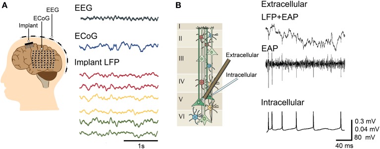
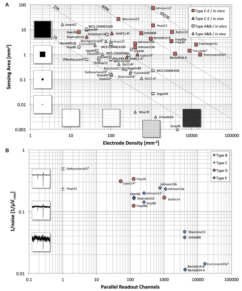
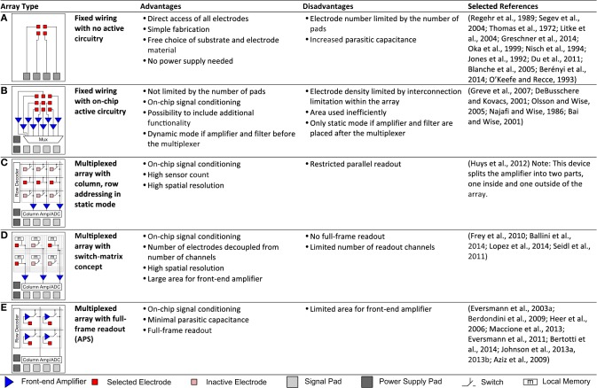
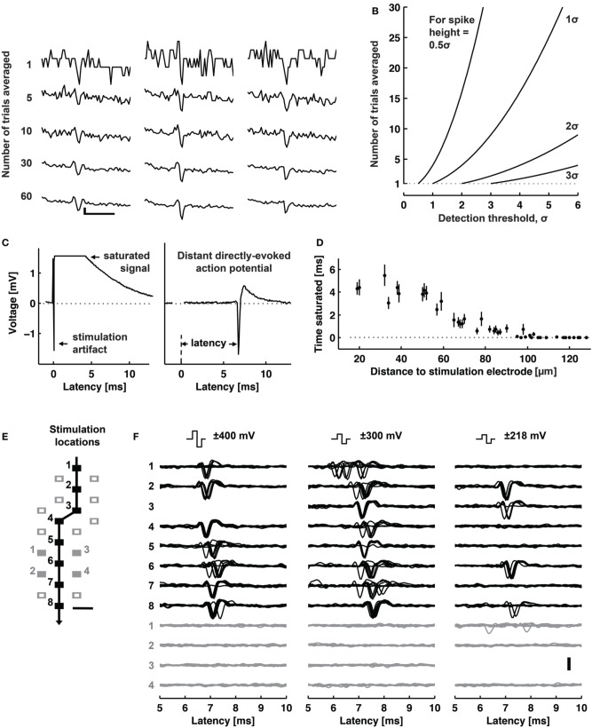
Microelectrode arrays and microprobes have been widely utilized to measure neuronal activity, both in vitro and in vivo. The key advantage is the capability to record and stimulate neurons at multiple sites simultaneously. However, unlike the single-cell or single-channel resolution of intracellular recording, microelectrodes detect signals from all possible sources around every sensor. Here, we review the current understanding of microelectrode signals and the techniques for analyzing them. We introduce the ongoing advancements in microelectrode technology, with focus on achieving higher resolution and quality of recordings by means of monolithic integration with on-chip circuitry. We show how recent advanced microelectrode array measurement methods facilitate the understanding of single neurons as well as network function.

Keywords: CMOS; extracellular recording; microelectrode array; multi-scale modeling; multielectrode array; neuron-electrode interface; neuronal function; stimulation.

Figure 1

Typical electrophysiological methods. (A) Macroscopic recording via electroencephalography (EEG) and mesoscopic recording through electrocorticography (ECoG) and implantable electrodes, with the corresponding representative waveforms recorded in a patient with drug-resistant epilepsy. The measured signal amplitudes are larger for ECoG and implanted electrodes (local field potential or LFP recording) compared to EEG. The waveforms for EEG, ECoG, and implant are modified with permission from Buzsáki et al. (2012). (B) Mesoscopic and microscopic recording using a tetrode (extracellular) and a glass micropipette (intracellular), respectively. The fast EAP extracted from the raw tetrode recordings correlate with the intracellular APs recorded from a pyramidal cell. (Left) Illustration of cells across cortical layers modified with permission from Buzsáki et al. (2012). (Right) Signals for simultaneous extracellular and intracellular recordings modified with permission from Henze et al. (2000).

Figure 2

Device comparison. MEA comparison with respect to (A) electrode density and total sensing area, and (B) parallel recording channel count and noise level. (A) For devices with a regular sensor pitch, such as most in vitro MEA devices, the total area is calculated as number of electrodes times the pixel area. For all devices, the number of electrode times the inverse of the electrode density matches the total area. The light gray lines illustrate the number of electrodes. (B) The noise values shown are approximated RMS values stated in the respective citations. The conditions under which these measurements were taken usually differ significantly (such as noise bandwidth, in- or exclusion of electrode noise, inclusion of ADC quantization noise, etc.). Therefore, this graph only serves as a rough comparison. The waveforms to illustrate the noise levels are simulated and have a spectrum typical for MEA recordings. The simulated spikes are typical spikes for acute brain slice measurements recorded with microelectrodes. The recorded amplitudes may vary significantly depending on preparation and sensor characteristics. See Footnotes:,,,,.

Figure 3

Array architectures. This table summarizes and classifies the different architectures that are typically used for MEAs. Advantages, disadvantages are stated and representative selected references given. (A,B) Fixed wiring. (A) Electrodes are directly connected to signal pads with no active circuitry. (B) Electrodes are directly connected to on-chip active circuitry for signal conditioning. (C–E) Multiplexed arrays. (C) Signals are multiplexed to the signal pads via column, row addressing in static mode. (D) More flexible addressing is achieved by adding more routing resources within the array in the switch-matrix mode. (E) All electrodes can be sampled at fast speeds in full-frame readout implemented in active pixel sensor (APS) MEAs.

Figure 4

Stimulation capability of high-resolution CMOS-based MEA. (A) Examples of evoked spikes detected at three sites (columns) along the same axon. The top row shows individual raw traces, and the other rows show traces averaged as indicated. Scale bars, 1 ms horizontal, 10 μV vertical. (B) The amount of averaging necessary to detect a spike with a given height (0.5–3 σ) with respect to the detection threshold. (C) Left: A raw voltage trace recorded at an electrode neighboring a stimulation electrode saturated for about 4 ms (flat line). Right: A raw voltage trace recorded at an electrode located 1.46 mm away from a stimulation electrode did not saturate. (D) The duration of a saturated signal occurring after stimuli is plotted vs. distance from the stimulation electrode (mean ± s.e.m.; N = 18 stimulation electrodes from five CMOS-based MEAs). Stimuli consisted of biphasic voltage pulses between 100 and 200 ms duration per phase and between ± 400 and 800 mV amplitude. (E) Locations of stimulation electrodes that directly evoked (black boxes) or did not evoke (empty or filled gray boxes) APs detected at a soma located ~890 μm away. The line arrow indicates the orthodromic propagation direction. Scale bar, 20 μm. (F) Voltage traces of somatic APs elicited by biphasic voltage stimuli. Traces in response to eight stimuli are overlaid for each of three stimulation magnitudes (indicated at the top), plotted for all effective (black) and four ineffective stimulation sites (gray at the bottom). Stimulation electrode locations are represented as numbered boxes in (E). Scale bar, 200 μV. All panels and description adapted with permission from Bakkum et al. (2013).

Figure 5

CMOS-based in vitro MEAs. CMOS-based in vitro MEAs, their key specifications and references to biological applications for recording and stimulation are listed in this table. The application list includes only one representative citation for each type of preparation. The specification for each device are taken from the reference listed on top and may differ for other versions of the device.

Figure 6

MEA stimulation and recording system diagram with the noise sources. The neuron is stimulated by the pulses or waveform generated digitally through the MEA. The response of the neuron, typically an action potential, is transformed by different parameters across the components of the MEA toward the recorded signal.

Figure 7

MEA neuron-electrode interface. (A) The classic point or area contact model derived from Fromherz (2003). The cell membrane is represented with an equivalent model based on the Hodgkin-Huxley model of the squid axon (Hodgkin and Huxley, 1952). C_M represents the capacitance across the neuronal membrane, i.e., the lipid bilayer. The voltage-gated ion channels (K for potassium and Na for sodium) are represented by non-linear conductances, g_K and g_Na, and the leak is shown as a linear conductance, g_L. The reversal potentials that drive the flow of ions are represented by E_K, E_Na, and E_L. The ion flow is shown by I_K, I_Na, I_L, and I_C. The other elements are described in the text. V_rec is the recorded voltage signal. Typical IAP and EAP recordings are shown. The location of the scissors indicates where the “cut” can be made to separate the neuron-electrode interface into two parts. (B) Generalized neuron-electrode interface separating the problem into two parts. Upper—“Fluid”-side: The potential at the electrode sites can be solved using the volume conductor theory. The MEA surface is assumed to be an insulator such that the method of images can be applied on Coulomb's law to solve the potential at any point on the MEA surface. The neuron-electrode distance influences the signal amplitude measured at the electrodes. High spatial resolution allows for recording at several locations of a single neuron, with large negative spikes located at the perisomatic area and positive spikes at the dendritic area, i.e., return current. Lower—“Metal”-side: The voltage measured at the electrode is shaped by the electrical parameters of the electrode-electrolyte interface, represented by Z′_e as the effective electrode impedance and Z′_a as the effective input impedance. This model is derived from Robinson (1968), Nelson et al. (2008), Hierlemann et al. (2011).

Figure 8

Neuronal culture studies using MEAs. (A,B) Combination of MEAs with immunostaining and microscopy to analyze the relationship between the development of synapses and electrical activity of neurons, adapted with permission from Ito et al. (2013). (A) Plot showing the number of synapses along the neuronal dendrites in a long-term primary culture. The glutamatergic (red) and GABAergic (green) synapses along the dendrites of neurons were obtained by immunostaining from cultures at 7–35 days in vitro (DIV). The number of synapses at the dendrites continuously increased for 3 weeks and saturated afterwards. The same is true for synapses at the soma (not shown), which saturated after 30 DIV. (B) Plotted data from MEA recordings of a long-term culture. A similar pattern is observed from the firing rate and synchronized burst rate measured by a MED64 MEA device from 7 to 35 DIV. Both the firing and burst rates increased until 30 DIV, which eventually saturated afterwards. (C,D) Application of HDMEAs to analyze the functional connectivity of neurons in vitro, adapted with permission from Maccione et al. (2012). Fluorescent images of stained neurons on an HDMEA are shown with arrows indicating the functional connectivity (from white—weak to red—strong) obtained by analyzing spike trains using cross-correlation.

Figure 9

Waves in acute hippocampal slices revealed by MEAs. (A–C) Studying the effect of the delayed rectifier potassium channel α-subunit Kv1.1 to sharp waves in in vitro hippocampal slices using MEAs, modified with permission from Simeone et al. (2013). (A) Image of a Kcna1-null (knock-out of the gene encoding Kv1.1) hippocampal slice on an MEA. Black squares correspond to the electrodes. The regions of the hippocampus are also indicated. (B) The sharp waves in wild-type (WT) and Kcna1-null hippocampi are initiated in CA3 that spread with similar time-courses. (C) Representative sharp waves from WT and Kcna1-null hippocampi recorded at the location of red boxes in (A). The sharp waves are longer (with ripples) in Kcna1-null compared to WT. Scale bars: horizontal, 50 ms; vertical, 50 μV except for WT CA3sp (100 μV), WT CA3sr (200 μV), KO CA1sp (20 μV), and WT CA1sr (200 μV). CA, cornus ammonis; DG, dentate gyrus. (D,E) Studying the effect of deleting synapsin II (Syn II) to the tonic inhibition in mouse hippocampal slices using HDMEAs, adapted with permission from Medrihan et al. (2014). (D) Mean firing rate computed from each electrode from WT and Syn II knock-out hippocampal slices before and after THIP treatment. THIP: (4,5,6,7-tetrahydroisoxazolo[5,4-c]pyridin-3-ol; gaboxadol), a selective agonist of δ subunit-containing GABAA receptors. (E) Raster plots showing highly synchronized bursts, x-axis corresponds to time, y-axis corresponds to pixels (electrode). THIP reduced the high frequency bursts in Syn II knock-out hippocampus. Scale bar: 1 min.

Figure 10

High-resolution mapping of spontaneous Purkinje cell activity using HDMEAs. (A–E) HDMEA recordings from an acute slice preparation of the caudal half of the cerebellar vermis. (A) Activity map of the detectable spike activity in the recording area. Small dots correspond to the electrodes used for recording (~30% of the available electrodes). Events exceeding a threshold of ±36 μV were used to calculate the color-coded event rate. Scale bar: 0.3 mm. (B) Close-up of a region with high activity delimited in (A). All units identified by spike sorting are marked, i.e., the somatic region is blue and the dendritic region is red. Scale bar: 0.1 mm. (C) Schematic of the basic cellular structures in the cerebellar slice (Gray, 1918). Scale bar: 0.1 mm. ML, molecular layer; PCL, Purkinje cell layer; GL, granular layer; CF, climbing fiber; MF, mossy fiber; PF, parallel fiber; PC, Purkinje cell; GgC, Golgi cell; SC, stellate cell; BC, basket cell. (D) Footprint of a PC selected from the region shown in (B). Scale bar: vertical is 200 μV, horizontal is 1.9 ms. (E) Current source density (CSD) analysis for the cell shown in (D) at several points in time (green: sink; yellow: source). The sink moves from the soma at 0.4 ms to the proximal dendrites at 0.6 ms and covers the dendritic area, while the soma repolarizes. Frequency band: 180 Hz–3.5 kHz. (F–H) Matching simulated and measured EAP footprints. (F) Comparison of the recorded average single-unit spikes (black traces) and the spikes calculated from a compartment-model simulation of a PC (green traces). Scale bar: vertical is 100 μV, horizontal is 1.9 ms. (G) Illustration of the position and orientation of the simulated PC, with the center of the soma located [blue diamond in (F)] 40 μm above the chip surface. (H) Simulated potential on the chip surface along a line parallel to the soma-dendrite axis [dashed blue line in (F,G)] during the spike evolution at 0.1 ms intervals. The black and white dots on the potential line of maximal amplitude (bold blue line) represent the HDMEA spatial resolution (18 μm pitch). Significant spatial undersampling of the potential distribution curve can be observed by reducing the lateral spatial resolution by 50% (black dots only, pitch 36 μm), especially for the largest negative peak. All panels and descriptions adapted with permission from Frey et al. (2009a).

Figure 11

Identification of retinal ganglion cell receptive fields using HDMEAs. (A–E) Characterization and analysis of HDMEA recordings from defined populations of mouse retinal ganglion cells (RGCs), adapted with permission from Fiscella et al. (2012). (A) Each trace shows the average (thick black lines) of the 959 superimposed EAPs (gray lines). The electrode locations are indicated in (B). The propagation speed of the spike was calculated to be 0.7 m/s. (B) Footprint of an RGC over an area of 0.025 mm². The highest peak-to-peak amplitude is shown by the thick dark waveform. (C–E) Physiological response of RGCs. Left panel: RGC footprint on a recording block of the HDMEA. The yellow square indicates the location of the light stimulus, with the gray squares indicating the center of the stimulus at four positions. Middle panel: Raster plots corresponding to four stimulation locations indicated in the left panel. Each dot corresponds to a single EAP. Each raster plot shows the response to five repetitions of the same stimulus. The firing rate of the RGC (averaged from five responses) is indicated below. Right panel top: Polar plot showing the responses of the RGC to motion of a bar in 8 directions at 45° radial intervals. Right panel bottom: Inter-spike interval distribution showing the time intervals between consecutive spikes. (C) Blue = ON RGC. (D) Red = OFF RGC. (E) Green = ON-OFF RGC. (F) Classification of RGC types and receptive fields at single cone resolution, adapted with permission from Field et al. (2010). The RGCs were recorded simultaneously and classified using the responses to white noise stimuli. Top middle panel: Receptive field radius vs. the first principal component of the response time course. The clusters reveal different RGC types. Surrounding panels: Identified RGC types highlighted at the top middle panel. The RGCs are stimulated with fine-grained white noise to reveal single cone receptive fields. Scale bars: 50 μm.

Figure 12

Imaging axonal signal propagation using HDMEAs. (A–C) Axonal propagation of a cultured neuron on an HDMEA, adapted with permission from Bakkum et al. (2013). (A) Live image of a neuron at 21 DIV transfected with red fluorescent protein (RFP). The axon is highlighted. (B) Illustration of the distributed stimulation method. The crosshair represents the location of the “somatic” AP observed while stimulating different electrodes represented by colored dots (color represent the median latency until AP detection, where light gray corresponds to electrodes that did not evoke an AP). The small dots represent the location of the HDMEA electrodes. Scale bar, 40 μm. (C) Illustration of the single-site stimulation method. The red crosshair represents the stimulated electrode. The colored dots represent the latencies of detected APs with respect to the largest voltage signal indicated by the arrow. Scale bar, 40 μm. (D) Axonal propagation of an RGC from rabbit retina, adapted with permission from Zeck et al. (2011). Consecutive electrical images of the EAP propagation allow for the calculation of axonal conduction velocity. (a) Image of a somatic AP (blue spot in the first window) propagating along the proximal axon. (b) Image of a biphasic spike recorded from an axon. (c) Plot indicating the distance traveled of the AP in time. Open symbols represent data calculated from recordings at 16.4 kHz; closed symbols are recordings at 8.2 kHz.

Figure 13

Localization of single neurons. (A) Spike current source density (sCSD) method by Somogyvári et al. (2012), figure modified with permission. The experimental setup is shown on the left, where the neuron is oriented at a distance d parallel to the in vivo MEA. The highest amplitude comes from the current sources at the soma of the neuron (sink) and is detected by multiple electrodes. The forward solution at d is given by the T(d) matrix, which transforms the CSD on the neuron to the EAP detected by the MEA. The EAPs are shown in the voltage traces per electrode, where one spike is plotted as a color map, indicating the spatial EAP pattern in time. The sCSD obtained from the EAP signals by inverse solution T⁻¹(d_opt) is shown on the right. The EAP spatio-temporal map is transformed into a series of normalized CSD distributions [I(d)] with different d-values. Localization is done by solving for d_opt. The optimum d (d_opt) is chosen as the value where I(d) is the most spike-like, i.e., similar to the normalized amplitude of the EAP during the whole duration of the spike. Thus, the EAP and sCSD color maps are similar. (B–D) Localization of simulated neurons using simplified line model by Delgado Ruz and Schultz (2014), figures adapted with permission. (B) The simulated neurons are CA1 pyramidal, L2/3 pyramidal, double bouquet or DB (not shown), NPY interneurons, and PV interneuron. Localization depends on the location of the sodium trough, which corresponds to the moment when currents are concentrated near the soma. As shown by the color map embedded on the neuron morphologies, the sodium trough (red) is displaced from the soma for NPY due to the contribution of the dendritic arbor and axon, leading to higher localization error along the Y axis shown in (D). (C) Localization results for CA1, where the errors along X–Z axes remained low for neuron-electrode distances under 35 μm and increased thereafter, especially along the Z axis. (D) The localization errors were not similar for all simulated neurons. The differences in morphology and electrophysiology cause the errors, although the maximum EAP (location of sodium trough) is more or less confined to the perisomatic area.

Figure 14

Ion channel density estimation. Adapted from Gold et al. (2006). (A) The extracellular action potentials (EAPs) solved in a grid from the multicompartmental model of a CA1 pyramidal neuron. The dotted black line indicates the tip of the electrode used to measure the EAPs. (B) Enlarged image of the EAP at the electrode tip. Location is indicated by the white dotted line in (A). Solid line in the plot corresponds to the simulated EAP, which is superimposed with the recorded EAP shown as dotted line. (C) Comparison of the simulated intracellular signal (solid line) at the proximal apical trunk to the intracellular recording (dotted line). (D) First column: The details of the intracellular signal simulation for each compartment. White solid lines in (A) indicate the locations of the compartments. Second column: The simulated membrane currents in the same compartments as the first column. The net membrane current across the soma and proximal dendrites best estimates the EAP waveform. Third column: Membrane current components in terms of Na⁺, K⁺, and mixed-ion capacitive current. Last column: Conductivity densities of the A, C, D, K, and M type K⁺ currents. For further details, see Gold et al. (2006).

References

1. Abel T., Havekes R., Saletin J. M., Walker M. P. (2013). Sleep, plasticity and memory from molecules to whole-brain networks. Curr. Biol. 23, R774–R788. 10.1016/j.cub.2013.07.025 - DOI - PMC - PubMed
1. Abeles M., Gerstein G. L. (1988). Detecting spatiotemporal firing patterns among simultaneously recorded single neurons. J. Neurophysiol. 60, 909–24. - PubMed
1. Ahuja A. K., Dorn J. D., Caspi A., McMahon M. J., Dagnelie G., Dacruz L., et al. . (2011). Blind subjects implanted with the Argus II retinal prosthesis are able to improve performance in a spatial-motor task. Br. J. Ophthalmol. 95, 539–543. 10.1136/bjo.2010.179622 - DOI - PMC - PubMed
1. Anastassiou C. A., Buzsáki G., Koch C. (2013). Biophysics of extracellular spikes, in Principles of Neural Coding, eds. Quiroga R., Panzeri S. (Boca Raton, FL: CRC Press; ), 15–36 10.1201/b14756-4 - DOI
1. Andersen R. A., Hwang E. J., Mulliken G. H. (2010). Cognitive neural prosthetics. Annu. Rev. Psychol. 61, 169–90, C1–C3. 10.1146/annurev.psych.093008.100503 - DOI - PMC - PubMed