Locally epistatic genomic relationship matrices for genomic association and prediction

Abstract

In plant and animal breeding studies a distinction is made between the genetic value (additive plus epistatic genetic effects) and the breeding value (additive genetic effects) of an individual since it is expected that some of the epistatic genetic effects will be lost due to recombination. In this article, we argue that the breeder can take advantage of the epistatic marker effects in regions of low recombination. The models introduced here aim to estimate local epistatic line heritability by using genetic map information and combining local additive and epistatic effects. To this end, we have used semiparametric mixed models with multiple local genomic relationship matrices with hierarchical designs. Elastic-net postprocessing was used to introduce sparsity. Our models produce good predictive performance along with useful explanatory information.

Keywords: GenPred; epistasis; genomic selection; mixed models; shared data resource.

Figure 1

A hypothetical hierarchical setup for an organism with three chromosomes. This division has two main parameters, namely the “depth” and the “nsplit.” Depth controls how many levels of splits should be performed. A depth of zero corresponds to the root of the tree, a depth of one corresponds to chromosomes, a depth of two corresponds to splitting the chromosomes, and so on. The nsplit parameter controls the number of divisions after the chromosome level. Here, a setup with depth two and nsplit three is illustrated.

Figure 2

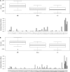
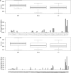
Wheat data: accuracies of the multiple-kernel (MK) model compared to the Gaussian (Gaus) kernel model for six traits. Circles below the line in red correspond to the cases where the MK model is more accurate than the Gaus model. (A) Two regions per chromosome. (B) Three regions per chromosome.

Figure 3

Wheat data: associations from the multiple-kernel (MK) model for the six traits. (A) Two regions per chromosome. (B) Three regions per chromosome.

Figure 4

Mouse data: accuracies and associations for multiple-kernel (MK) model and accuracies for linear kernel (Lin) and Gaussian kernel (Gaus) models for “weight at age of 6 weeks (grams).” (A) Four regions per chromosome. (B) Nine regions per chromosome.

Figure 5

Mouse data: accuracies and associations for multiple-kernel (MK) model and accuracies for linear kernel (Lin) and Gaussian kernel (Gaus) models for “growth slope between 6 and 10 weeks of age (grams per day).” (A) Four regions per chromosome. (B) Nine regions per chromosome.

Figure 6

Barley data: accuracies and associations for multiple-kernel (MK) (four regions per chromosome) model and accuracies for linear kernel (Lin) and Gaussian kernel (Gaus) models for tocotrienol levels.

Figure 7

Maize data: accuracies and associations for multiple-kernel (MK) (25 regions per chromosome) model and accuracies for linear kernel (Lin) and Gaussian kernel (Gaus) models for degree days to silking.

Figure 8

Maize data: accuracies for multiple-kernel (MK) (36 regions per chromosome), linear kernel (Lin), and Gaussian kernel (Gaus) models for degree days to silking.

Figure 9

Simulations: accuracies of models are compared for traits that are generated by short-range to long-range interactions. On the horizontal axis the scenarios are displayed in increasing order from left to right with respect to the range of interactions ($1,4,10,20,30$, and 50 cM and genome-wide). The vertical axis displays the accuracy.

Figure 10

Simulations: four measures of classification model performance averaged over the 100 replications for sample sizes 500, 750, 1000, and 1500 and multiple-kernel models with 10, 20, 30, 40, or 50 splits per chromosome.

Figure 11

Simulations: the estimated prediction accuracies (measured by correlation, r) by cross-validation in the training set for number of splits = 1–10 and estimated prediction accuracies in the test set for the same splits. The red vertical dotted line indicates the correct number of splits for each case.

References

1. Akdemir, D., and O. U. Godfrey, 2014 EMMREML: Fitting Mixed Models with Known Covariance Structures R Package Version 2.0. Available at: http://CRAN.R-project.org/package=EMMREML.
1. Amemiya T., 1977. A note on a heteroscedastic model. J. Econom. 6(3): 365–370.
1. Bach, F. R., G. R. Lanckriet, and M. I. Jordan, 2004 Multiple kernel learning, conic duality, and the SMO algorithm, p. 6 in Proceedings of the Twenty-First International Conference on Machine Learning. ACM., New York, NY DOI: 10.1145/1015330.1015424.
1. Blanchard G., Geman D., 2005. Hierarchical testing designs for pattern recognition. Ann. Stat. 33: 1155–1202.
1. Breitling R., Li Y., Tesson B. M., Fu J., Wu C. et al, 2008. Genetical genomics: spotlight on QTL hotspots. PLoS Genet. 4(10): e1000232. - PMC - PubMed
Publication types
LinkOut - more resources