The Strehler-Mildvan correlation from the perspective of a two-process vitality model

Abstract

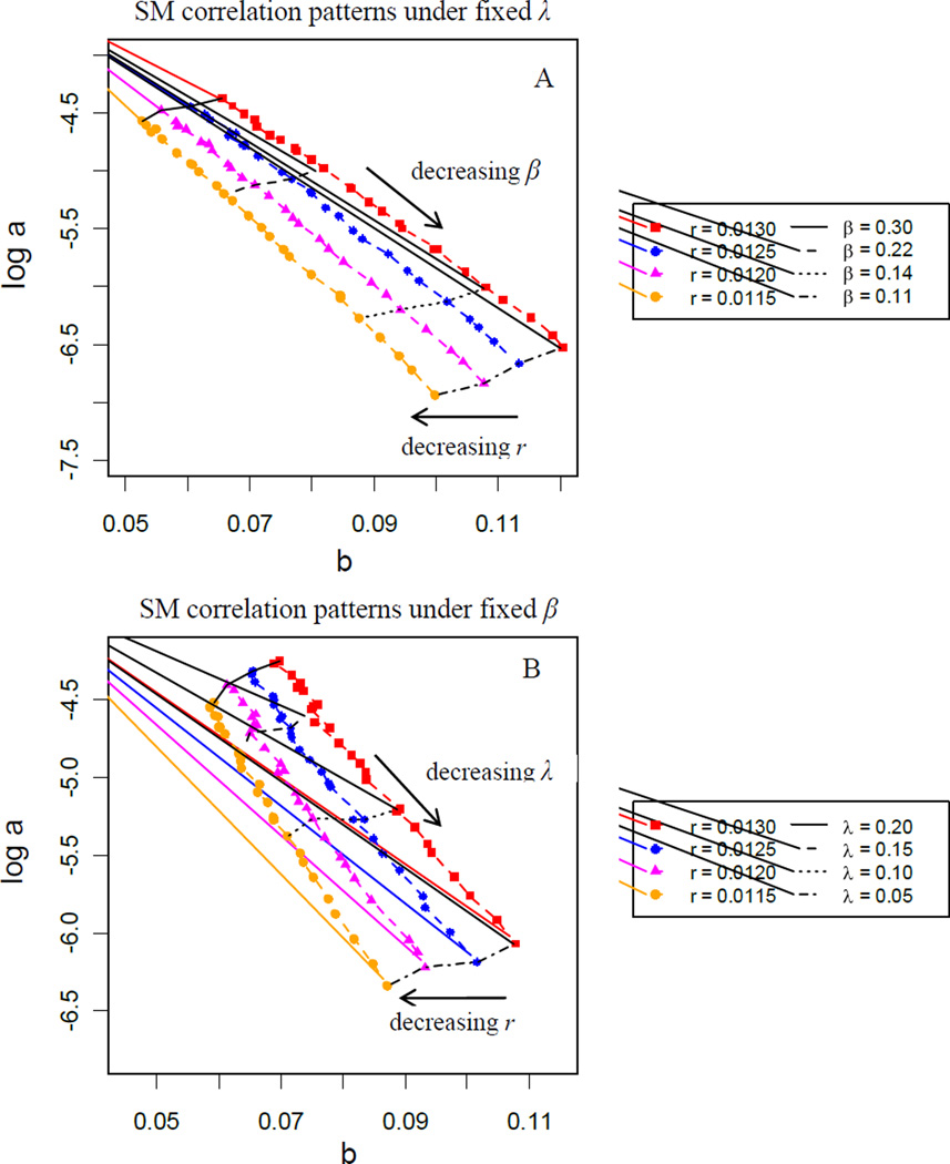
The Strehler and Mildvan (SM) general theory of ageing and mortality provides a mechanism-based explanation of Gompertz's law and predicts a log-linear relationship between the two Gompertz coefficients, known as the SM correlation. While the SM correlation is supported by data from developed countries before the second half of the twentieth century, the recent breakdown of the correlation pattern in these countries has prompted demographers to conclude that SM theory needs to be reassessed. In this paper we use a newly developed two-process vitality model to explain the SM correlation and its breakdown in terms of asynchronous trends in acute (extrinsic) and chronic (intrinsic) mortality factors. We propose that the mortality change in the first half of the twentieth century is largely determined by the elimination of immediate hazards to death, whereas the mortality change in the second half is primarily driven by the slowdown of the deterioration rate of intrinsic survival capacity.

Keywords: Gompertz coefficients; SM correlation; intrinsic and extrinsic mortality; mortality pattern; vitality.

Figure 1

(A) Female Period: patterns of SM correlation in France (1861–2005), Sweden (1861–2005), Japan (1950–2000) and the US (1938–2005); (B) Female Cohort: patterns of SM correlation in France (1859–1917), Sweden (1821–1915) and the US (1883–1927). Note: For consistency with other studies (see Fig. 3 and Fig. 5 in Yashin et al. (2001a)), we used mortality for ages between 40 and 80. Source: Human Mortality Database (2011).

Figure 2

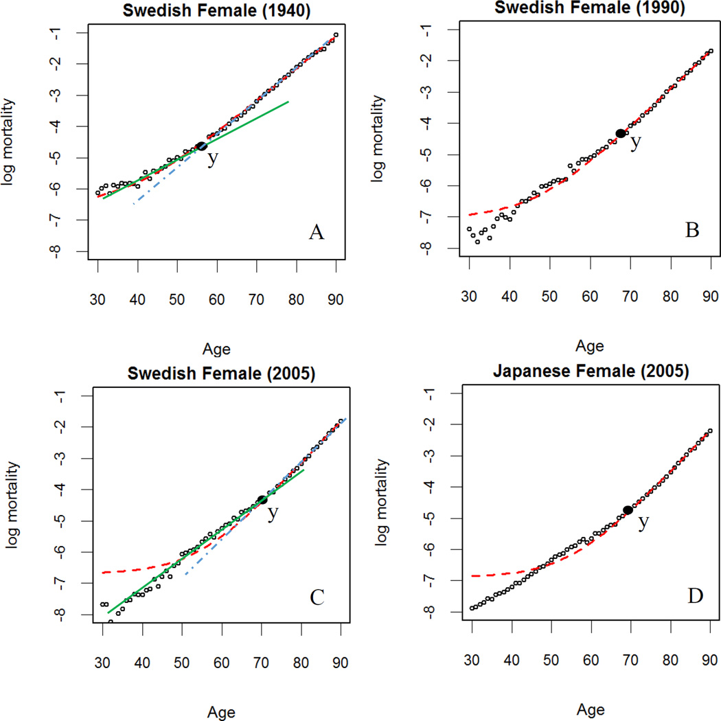
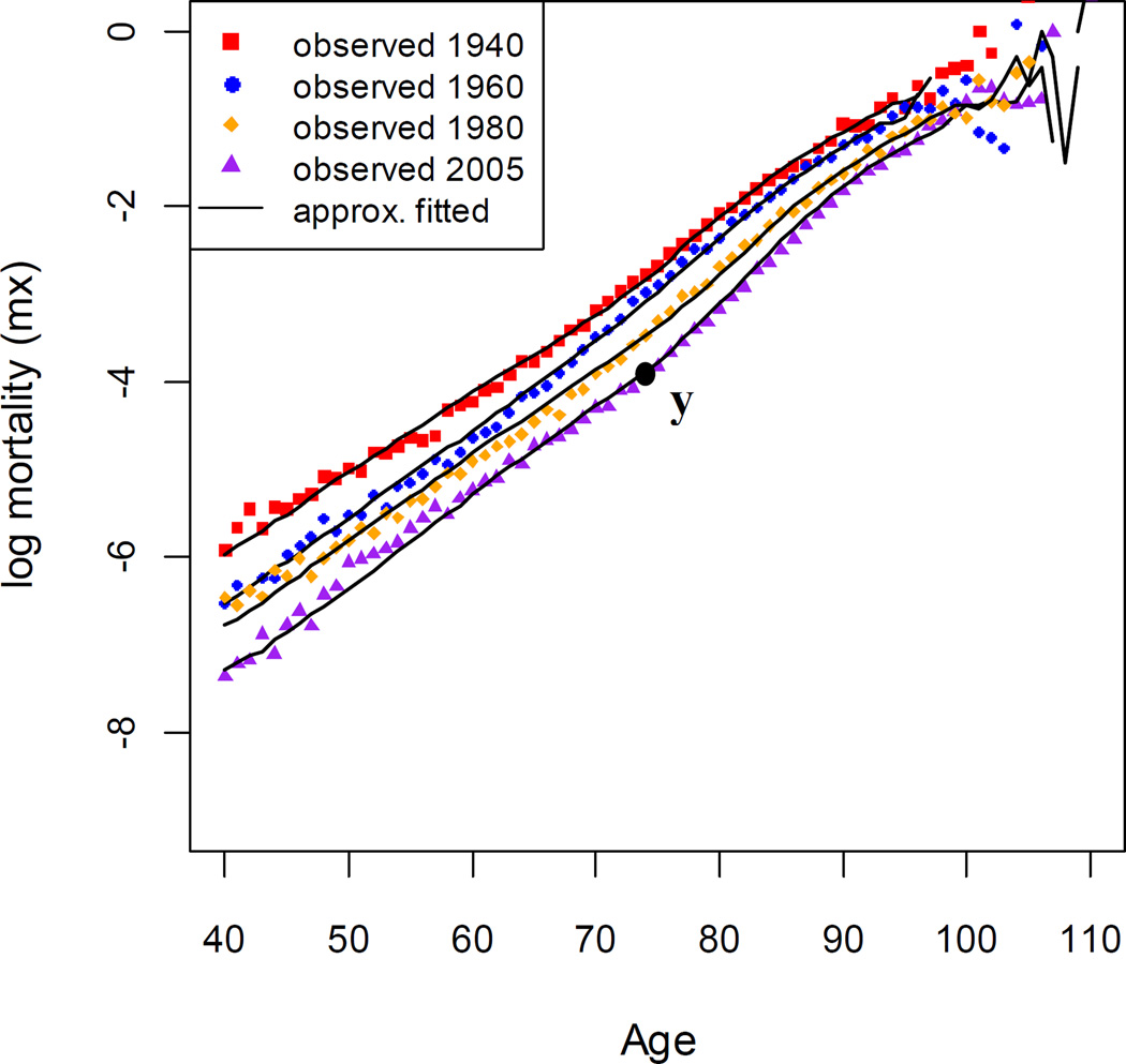
Gompertz-Makeham model fit to selected period mortality data. (A): Swedish Female, 1940; (B) Swedish Female, 1990; (C) Swedish Female, 2005; (D): Japanese Female, 2005. Note: The data (○) is fit with the GM model () using conventional weighted least-squares methods. A piecewise linear model that transitions between the middle-age () and old-age () linear segments at age y was demonstrated in (A) and (C). Source: As for Figure 1.

Figure 3

Gompertz-Makeham background mortality (M) derived by weighted least-squares of fitting period data for Swedish females between ages 30 and 90. Source: As for Figure 1.

Figure 4

The two-process vitality model illustrated. Note: Vitality declines stochastically from an initial value of 1. Intrinsic mortality results when adult vitality is exhausted, ①, and extrinsic mortality occurs when a random challenge exceeds the remaining vitality, ② (Reproduced from Fig. 1 of Li and Anderson (2013)).

Figure 5

The approximated fit of the two-process vitality model to selected period mortality curves of Swedish females (40–110). Note: The approximated parameter values are 1940 (r = 0.0177, s = 0.0112, λ = 0.155, β = 0.202), 1960 (r = 0.0175, s = 0.011, λ = 0.152, β = 0.171), 1980 (r = 0.0164, s = 0.0102, λ = 0.142, β = 0.172), and 2005 (r = 0.0161, s = 0.010, λ = 0.12, β = 0.157). Source: As for Figure 1.

Figure 6

Simulated SM correlation patterns. Note: (A) Mortality curves are all simulated under fixed challenge frequency term λ = 0.12; (B) Mortality curves are all simulated under fixed challenge average magnitude term β = 0.125. For both (A) and (B), curves all have the same background variance structure in vitality: s = 0.01.

Figure 7

Simulated patterns of log mortality under varying values of the two-process vitality model parameters. Note: (A) r changes while s, λ, and β are fixed at 0.012, 0.150 and 0.167 respectively; (B) s changes while r, λ, and β are fixed at 0.0165, 0.150 and 0.167 respectively; (C) λ changes while r, s, and β are fixed at 0.0165, 0.012 and 0.167 respectively; (D) β changes while r, s, and λ are fixed at 0.0165, 0.012 and 0.150 respectively.

References

-
- Aalen OO, Gjessing HK. Understanding the shape of the hazard rate: a process point of view. Statistical Science. 2001;16(1):1–13.
- Anderson JJ. A vitality-based model relating stressors and environmental properties to organism survival. Ecological Monographs. 2000;70(3):445–470.
- Anderson JJ, Gildea MC, Williams DW, Li T. Linking growth, survival, and heterogeneity through vitality. The American Naturalist. 2008;171(1):E20–E43. - PubMed
- Bongaarts J. Long-range trends in adult mortality: Models and projection methods. Demography. 2005;42(1):23–49. - PubMed
- Borgan O, Gjessing HK, Gjessing S. Survival and Event History Analysis: A Process Point of View. Dordrecht: Springer; 2008.
Publication types
MeSH terms
Grants and funding
LinkOut - more resources
Full Text Sources
Other Literature Sources