. 2015 Feb 19;518(7539):399-403.
doi: 10.1038/nature14182. Epub 2015 Feb 4.

Functional organization of excitatory synaptic strength in primary visual cortex

Affiliations

Functional organization of excitatory synaptic strength in primary visual cortex

Lee Cossell et al. Nature. .

Abstract

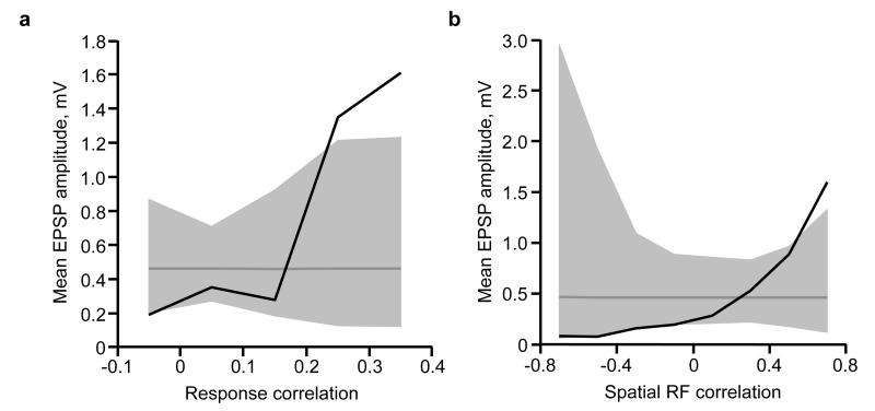
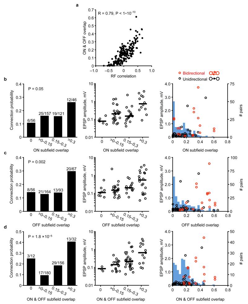
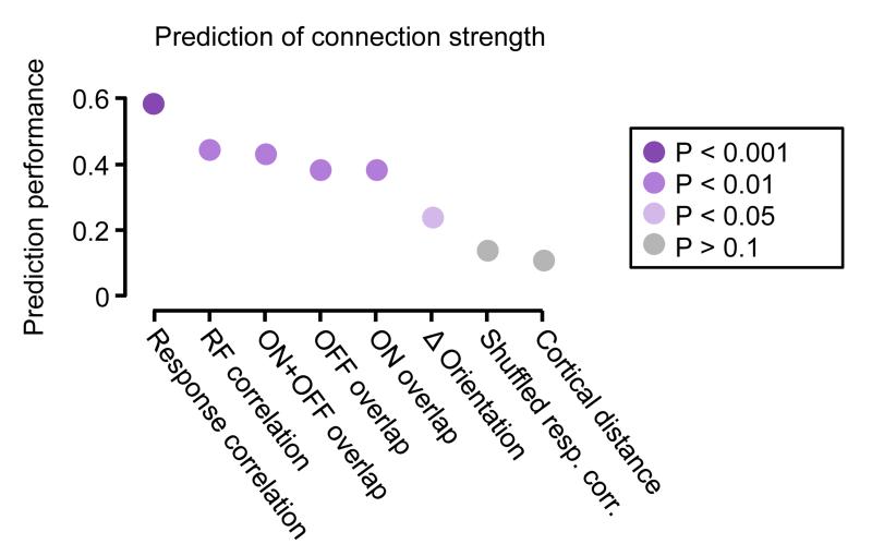
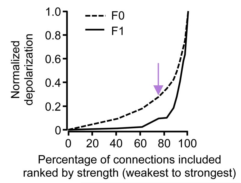
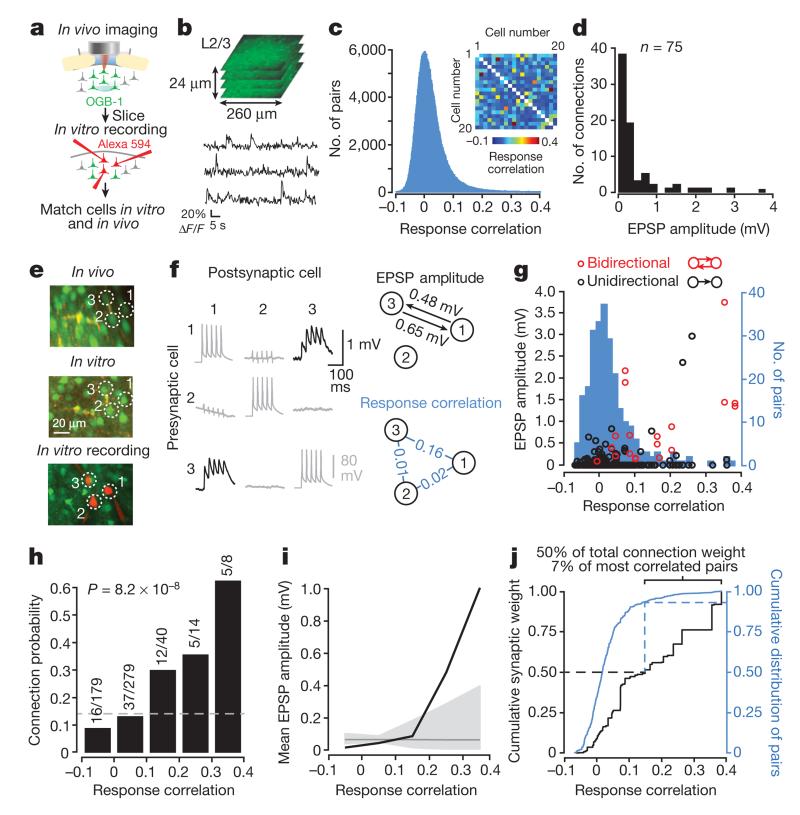
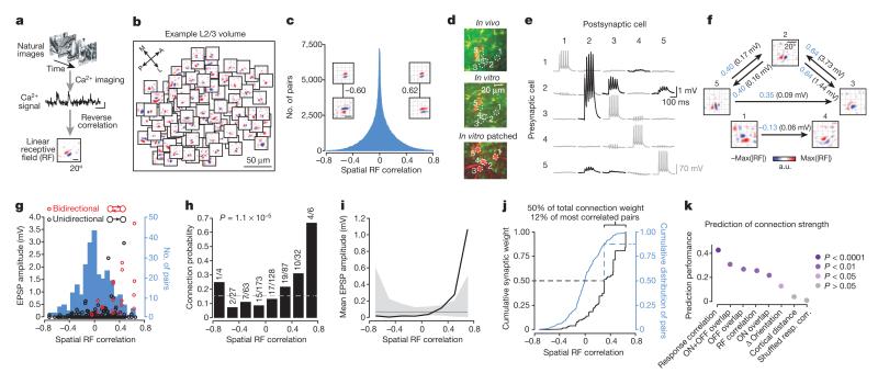
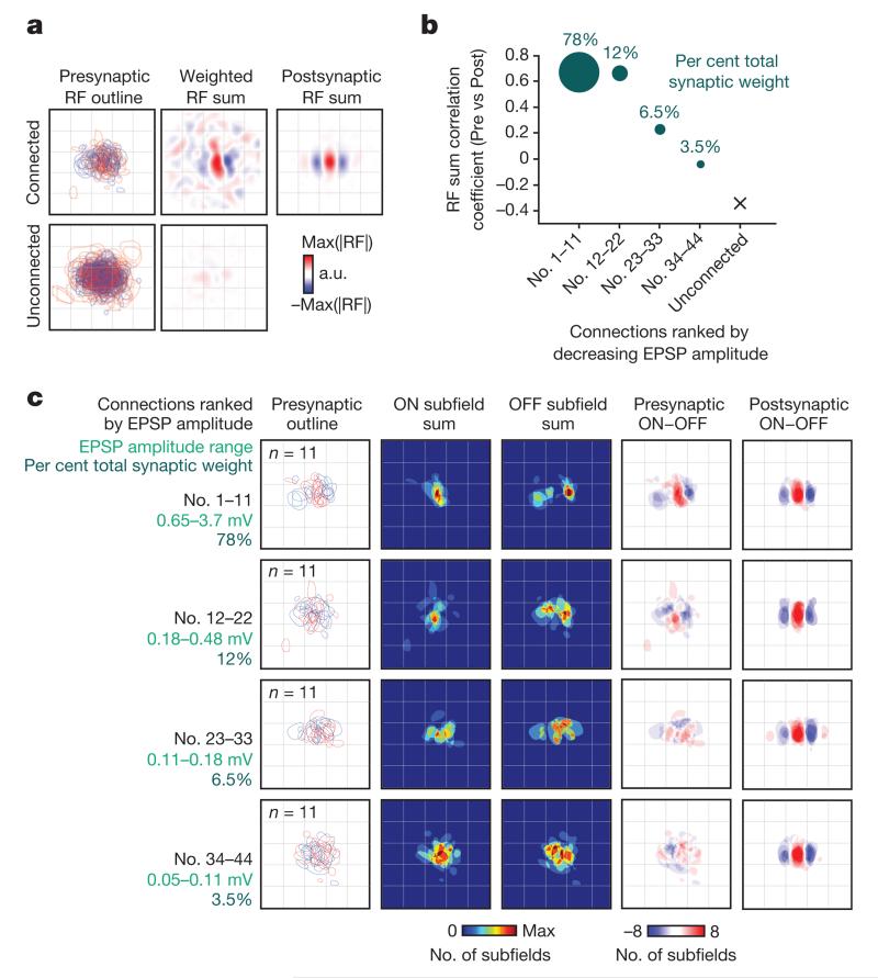
The strength of synaptic connections fundamentally determines how neurons influence each other's firing. Excitatory connection amplitudes between pairs of cortical neurons vary over two orders of magnitude, comprising only very few strong connections among many weaker ones. Although this highly skewed distribution of connection strengths is observed in diverse cortical areas, its functional significance remains unknown: it is not clear how connection strength relates to neuronal response properties, nor how strong and weak inputs contribute to information processing in local microcircuits. Here we reveal that the strength of connections between layer 2/3 (L2/3) pyramidal neurons in mouse primary visual cortex (V1) obeys a simple rule--the few strong connections occur between neurons with most correlated responses, while only weak connections link neurons with uncorrelated responses. Moreover, we show that strong and reciprocal connections occur between cells with similar spatial receptive field structure. Although weak connections far outnumber strong connections, each neuron receives the majority of its local excitation from a small number of strong inputs provided by the few neurons with similar responses to visual features. By dominating recurrent excitation, these infrequent yet powerful inputs disproportionately contribute to feature preference and selectivity. Therefore, our results show that the apparently complex organization of excitatory connection strength reflects the similarity of neuronal responses, and suggest that rare, strong connections mediate stimulus-specific response amplification in cortical microcircuits.


Figures

<b>Extended Data Figure 1</b>.
Extended Data Figure 1.. Relationship between response correlation coefficient or RF correlation and cortical distance
a, Pairwise response correlation coefficient plotted as a function of cortical distance, for an example region, indicates only a weak relationship between response correlation and cortical distance (R = −0.06). Red line denotes mean value of response correlation in 50 μm bins of cortical distance. b, Pairwise RF correlation plotted as a function of cortical distance, for the same example region as in a. Again, only a weak relationship was observed (R = −0.02).
<b>Extended Data Figure 2</b>.
Extended Data Figure 2.. Relationship between mean connection amplitude and response correlation or RF correlation
a, Black trace, mean connection amplitude (excluding unconnected pairs) plotted against response correlation. Dashed grey line indicates mean EPSP amplitude of all connections. Grey shaded region represents the 95% confidence interval of the expected mean, estimated by repeated random reshuffling of the EPSP amplitudes among all cell pairs in the data set. Connections were binned with ranges from −0.1 to 0, 0 to 0.1, and so on. b, Black trace, mean connection amplitude (excluding unconnected pairs) plotted against RF correlation. Dashed grey line indicates mean EPSP amplitude of all connections. Grey shaded region represents the 95% confidence interval of the expected mean, estimated by repeated random reshuffling of the EPSP amplitudes among all cell pairs in the data set. Connections were binned with ranges from −0.8 to −0.6, −0.6 to −0.4, and so on.
<b>Extended Data Figure 3</b>.
Extended Data Figure 3.. Relationship between connectivity and RF subfield overlap
a, The amount of ON and OFF subfield overlap (see Methods) was strongly correlated to the overall RF similarity as measured by RF correlation (R = 0.79, P < 1 × 10⁻¹⁰). b, Left panel, connection probability increased with increasing ON subfield overlap (P = 0.05; Cochran–Armitage test). Middle panel, EPSP amplitudes categorized into bins of ON overlap. Black line, median EPSP amplitude for each bin. Right panel, EPSP amplitude plotted against ON overlap. Red data points, bidirectional connections. Black data points, unidirectional connections. Underlying histogram shows frequency of recorded cell pairs as a function of ON overlap. c, Same as b, but for OFF overlap (P = 0.002; Cochran–Armitage test). d, Same as b, but for combined ON and OFF overlap (P = 1.8 × 10⁻⁵; Cochran–Armitage test). P values from the Cochran–Armitage test. To perform the Cochran–Armitage test, the bins at 0 and >0–0.15 were considered together, so that groups were evenly spaced.
<b>Extended Data Figure 4</b>.
Extended Data Figure 4.. Similarity of shared neuronal properties ranked according to how well they predict connection amplitude, when excluding unconnected pairs
Prediction performance and P values were calculated using a Monte-Carlo analysis (see Methods). Colours of the discs indicate P values.
<b>Extended Data Figure 5</b>.
Extended Data Figure 5.. Relationship between bidirectional and unidirectional connections and RF properties
a, EPSP amplitude plotted against RF correlation from bidirectionally (red) and unidirectionally connected pairs (black). Replotted from Fig. 2g. b, EPSP amplitude for bi- or unidirectional connections. Bidirectional connections were stronger than unidirectional connections (median connection amplitude: 0.44 mV for bidirectional connections, n = 22; 0.16 mV for unidirectional connections, n = 50; P = 4.4 × 10⁻⁴, Wilcoxon rank-sum test). c, RF correlation for bidirectionally connected, unidirectionally connected and unconnected pairs. The RFs of bidirectionally connected pairs were more correlated than those of unidirectionally connected or unconnected pairs (median RF correlation: 0.3 for bidirectionally connected pairs, n = 11; 0.04 for unidirectionally connected pairs, n = 50; P = 0.002; and −0.02 for unconnected pairs, n = 191, P = 5.3 × 10⁻⁵), although unidirectionally connected pairs did not have higher RF correlations than unconnected pairs (P = 0.18, Wilcoxon rank-sum test). d, Mean EPSP amplitude versus RF correlation for all (yellow), unidirectionally (black) or bidirectionally (red) connected pairs. There was a positive relationship between RF correlation and connection amplitude for both unidirectional and bidirectional connections.
<b>Extended Data Figure 6</b>.
Extended Data Figure 6.. Method of RF normalization
a, We normalized postsynaptic RFs to a template RF that was a vertical Gabor with 0 degree phase and an arbitrary but fixed spatial frequency (far right). A Gabor was fit to the RF of each postsynaptic neuron, and then rotated, translated and scaled so that the ON subfield was centred on the template’s ON subfield and the spatial frequencies matched. The same transformation was applied to presynaptic RFs of any simultaneously patched neurons. b, Transformation of the RF from an example postsynaptic neuron (upper row), and for the RF for its connected presynaptic neuron (middle row). Bottom row shows presynaptic RF outline overlaid on the postsynaptic RF at each step in the transformation.
<b>Extended Data Figure 7</b>.
Extended Data Figure 7.. Overlay of RFs between connected neurons
Presynaptic RF outline overlaid on the postsynaptic RF for all the connected pairs after performing normalization of the pre- and postsynaptic RFs to the RF template (n = 45). Numbers indicate connection amplitude.
<b>Extended Data Figure 8</b>.
Extended Data Figure 8.. Overlay of RFs between unconnected neurons
Assessed presynaptic RF outlines overlaid on the assessed postsynaptic RF for a representative set of unconnected pairs after normalization to the RF template.
<b>Extended Data Figure 9</b>.
Extended Data Figure 9.. Contribution of strong and weak connections to membrane potential depolarization
Removal of an increasingly larger fraction of the strongest inputs from the L2/3 model steeply reduces the large modulation component (F1) but more gradually reduces the mean depolarization component (F0). Model from Fig. 4d. Purple arrow indicates the weakest 75% of connections, as shown in Fig. 4i, j.
Figure 1
Figure 1. Excitatory connection strength reflects the similarity of pyramidal cell firing in vivo
a, Schematic of experimental protocol. b, Somatic calcium signals were sampled simultaneously from all neurons within a small volume of cortex (~260 × 260 × 24 μm). Two such volumes were recorded in each experiment. c, The distribution of pairwise response correlation coefficients for all imaged cell pairs. Inset, example matrix of correlation coefficients of pairwise responses from 20 neurons within a single imaged volume. d, Distribution of excitatory postsynaptic potential (EPSP) amplitudes (n = 75 connections). e, Example triplet of neurons shown in a transformed in vivo image (upper), in the brain slice (middle) and during whole-cell recordings (lower). f, Left, average postsynaptic potential traces of neurons in e. Black traces, connected; grey traces, unconnected; evoked presynaptic spikes are along the diagonal. In some traces, capacitative stimulation artefacts coincide with presynaptic spikes. Right, synaptic connectivity and response correlation coefficients of neurons in e. g, EPSP amplitude plotted against pairwise response correlation coefficient for bidirectionally (red) and unidirectionally (black) connected pairs. Underlying histogram shows the distribution of pairwise response correlation coefficients (blue, right y axis). h, Relationship between connection probability and pairwise response correlation. Grey dashed line, mean connection probability. Connection probability increased with response correlation (P = 8.2 × 10⁻⁸; Cochran–Armitage test). i, Mean connection amplitude (including unconnected pairs) plotted against response correlation (bin size = 0.1). Grey line, mean EPSP amplitude of all pairs. Grey shaded region represents the 95% confidence interval of the expected mean, estimated by repeated random reshuffling of the EPSP amplitudes among all cell pairs in the data set. j, Black trace, cumulative distribution of synaptic weight with respect to response correlation. A value of 1 corresponds to the linear sum of all EPSPs (33.34 mV). Blue trace, cumulative distribution of pairwise response correlation coefficients (right y axis).
Figure 2
Figure 2. Organization of excitatory connection strength with respect to linear RF properties
a, RFs obtained by regularized reverse correlation of responses to a sequence of static natural images (see Methods; scale bars: calcium trace, 20% ΔF/F, 5 s, RF, 20°). b, RFs distributed across an example imaged region (collapsed over cortical depth, 150–174 μm below cortical surface), revealing a large diversity of RFs. c, Distribution of spatial RF correlation coefficients for all recorded cell pairs. Inset, example RFs for two pairs of neurons and their correlation coefficients. Typically, negatively correlated RFs had similar orientation but opposite phase preference. d, Example quintuplet of neurons shown in the transformed in vivo image (upper), in the brain slice (middle) and during whole-cell recordings (lower). e, Average postsynaptic potential traces of neurons in d. Black traces, connected; grey traces, unconnected; evoked presynaptic spikes are along the diagonal. f, Synaptic connectivity and RFs of neurons in d. Arrows indicate a synaptic connection. Values indicate the correlation coefficient of RF maps (blue) and the amplitude of the connection (EPSP, black). a.u., arbitrary units. g, EPSP amplitude plotted against RF correlation for bidirectionally (red) and unidirectionally (black) connected pairs. Underlying histogram shows the distribution of pairwise RF correlations (blue, right y axis). h–j, Same as Fig. 1h–j for the RF correlation coefficient. k, Similarity of shared neuronal properties ranked according to how well they predict connection amplitude (including unconnected pairs). Prediction performance and P values were calculated using a Monte-Carlo analysis (see Methods). Disc colour indicates P value.
Figure 3
Figure 3. Combined synaptic input from the local L2/3 cortical network matches the RF structure of the receiving neuron
a, Top left, presynaptic RF outlines overlaid in normalized visual space (after rotation, translation and scaling of the postsynaptic RF; see text, Methods and Extended Data Fig. 7). Red outline indicates an ON subfield, blue outline indicates an OFF subfield. Bottom left, superimposed RF outlines for neurons assessed presynaptically, but which did not connect. Top middle, sum of presynaptic RFs. Each presynaptic RF was weighted by the EPSP amplitude from the pre- to the postsynaptic neuron. Bottom middle, RF sum for unconnected neurons assessed presynaptically. Top right, RF sum of the postsynaptic neurons. Before summing, each postsynaptic RF was weighted by the EPSP amplitude from the presynaptic to the postsynaptic neuron. b, Each point indicates the correlation between the presynaptic RF sum (weighted by the EPSP amplitude) and the corresponding postsynaptic RF sum, when including only connections in quarters of the connection amplitude distribution. The RF sum of the strongest 25% of inputs has the highest correlation with the postsynaptic RF (R = 0.67). This correlation value falls with decreasing connection strength. Disc area and values above represent the total synaptic weight accounted for by each quarter of the connection amplitude distribution. c, Relationship between ON and OFF subfields of connected pre- and postsynaptic neurons, ranked and displayed according to EPSP amplitude. Left column, presynaptic RF outlines of neurons grouped in quarters ranked by decreasing EPSP amplitude. Middle-left and middle columns, sum of binarized presynaptic ON and OFF subfields, respectively. Middle-right column, subtraction of summed OFF from summed ON subfields for presynaptic neurons. Right column, subtraction of summed OFF from summed ON subfields for postsynaptic neurons.
Figure 4
Figure 4. Simulation of local L2/3 excitatory input to single neurons qualitatively predicts the dynamics of membrane depolarization to drifting grating stimuli
a, Schematic of characteristic membrane potential (Vm) response to gratings drifting across a neuron’s RF in mouse V1. Both the preferred and the orthogonal stimuli evoke large membrane depolarizations (F0). Vm modulation (F1) is strongest when the grating and the RF are matched in orientation, and the grating cycles in and out of phase with the RF. b, Example in vivo whole-cell Vm recording from a L2/3 pyramidal cell during presentation of oriented gratings drifting in eight different directions. Black and grey arrows indicate preferred and orthogonal orientations, respectively. c, Average Vm response of the same neuron in b after spike removal. d, F0 and F1 components of Vm response to drifting gratings normalized to the preferred stimulus for neuron in b and c (left), and averaged across the population of recorded neurons (n = 24, right). e, Left, schematic of network model, showing input to a single L2/3 neuron from an example L2/3 neuronal population. Right, connection strengths were sampled from the experimentally measured relationship between EPSP amplitude and RF correlation (Fig. 2g). f, Responses for each presynaptic neuron were generated using a linear/nonlinear/Poisson model by correlating the visual input (drifting grating stimuli) with its experimentally measured RF (see Methods). Firing rates were weighted by their connection strengths (e) and summed to generate a time-varying Vm for each postsynaptic neuron. g, Example Vm response of a simulated neuron receiving input from the model L2/3 network. h, F0 and F1 components of the Vm response from the example simulated neuron in g (left) or from the population of simulated neurons (right, n = 4,633). i, Vm response of example simulated neuron in g when including only the strongest 25% of connections (top, blue trace) or weakest 75% of connections from the model network (bottom, purple trace). j, Same as d and h but for Vm responses driven by the strongest 25% of connections (blue) or weakest 75% of connections (purple).

Comment in

  • Neuroscience: The cortical connection.
    Scholl B, Priebe NJ. Scholl B, et al. Nature. 2015 Feb 19;518(7539):306-7. doi: 10.1038/nature14201. Epub 2015 Feb 4. Nature. 2015. PMID: 25652821 Free PMC article. No abstract available.

Similar articles

Cited by

References

    1. Markram H, Lübke J, Frotscher M, Roth A, Sakmann B. Physiology and anatomy of synaptic connections between thick tufted pyramidal neurones in the developing rat neocortex. J. Physiol. (Lond.) 1997;500:409–440. - PMC - PubMed
    1. Feldmeyer D, Lübke J, Sakmann B. Efficacy and connectivity of intracolumnar pairs of layer 2/3 pyramidal cells in the barrel cortex of juvenile rats. J. Physiol. (Lond.) 2006;575:583–602. - PMC - PubMed
    1. Holmgren C, Harkany T, Svennenfors B, Zilberter Y. Pyramidal cell communication within local networks in layer 2/3 of rat neocortex. J. Physiol. (Lond.) 2003;551:139–153. - PMC - PubMed
    1. Song S, Sjöström PJ, Reigl M, Nelson S, Chklovskii DB. Highly nonrandom features of synaptic connectivity in local cortical circuits. PLoS Biol. 2005;3:e68. - PMC - PubMed
    1. Lefort S, Tomm C, Floyd Sarria J, Petersen CH. The excitatory neuronal network of the C2 barrel column in mouse primary somatosensory cortex. Neuron. 2009;61:301–316. - PubMed

Publication types