Spatial information in large-scale neural recordings

Abstract

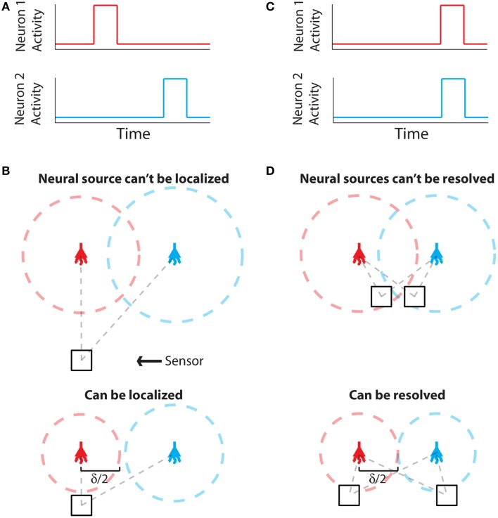
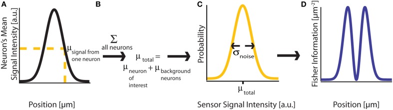
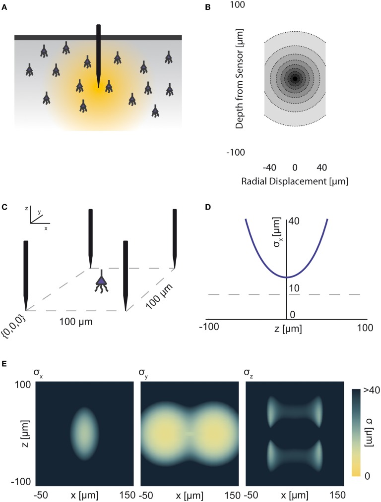
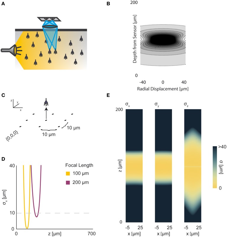
To record from a given neuron, a recording technology must be able to separate the activity of that neuron from the activity of its neighbors. Here, we develop a Fisher information based framework to determine the conditions under which this is feasible for a given technology. This framework combines measurable point spread functions with measurable noise distributions to produce theoretical bounds on the precision with which a recording technology can localize neural activities. If there is sufficient information to uniquely localize neural activities, then a technology will, from an information theoretic perspective, be able to record from these neurons. We (1) describe this framework, and (2) demonstrate its application in model experiments. This method generalizes to many recording devices that resolve objects in space and should be useful in the design of next-generation scalable neural recording systems.

Keywords: electrical recording; extracellular recording; fisher information; neural recording; optics; resolution; statistics; technology design.

Figure 1

Localization and Resolution. (A) In many behavioral states, neural systems have sparse activity, in which neighboring neurons (red and blue) are not active at the same time. In this scenario of single-source resolution, one neuron must be localized at a given time. (B) looks at this scenario. (B) Two neighboring neurons are shown a distance δ away from each other. Dotted lines indicate regions where we are confident about the source of a signal, i.e., we have a sufficient amount of information regarding that signal's location. The signals from the two neurons are recorded by the sensor at different times and do not interfere with each other. When a neuron cannot be localized effectively, i.e., there is not sufficient Fisher information, it is because the signal from that neuron was not strong enough to overcome noise. (C) Sometimes, neighboring neurons are simultaneously active. In this scenario of differential resolution, both neurons must be localized at a given time. (D) looks at this scenario. (D) Same as (B), except two sensors are necessary for differential resolution. When both sensors record similar signals, i.e., when there is large redundant information regarding the two neurons' activities, it is difficult to resolve the neurons.

Figure 2

Fisher Information. (A) A signal on sensor i from a neuron j at a particular location has a mean intensity, defined by a recording method's point spread function and the intensity of the signal from the active neuron. We here plot this mean signal intensity as a function of one position parameter. (B) The mean total signal on a sensor, μ_total, is the sum of the signals from every neuron. (C) The distribution of intensities recorded on a sensor is a function of the total mean signal, μ_total, and the variance of that signal, σ²_noise, which can result from many different noise sources. (D) Fisher information can be derived from the distribution of signal intensity values on a sensor.

Figure 3

Electrical Recording. An overview of the modeling and Fisher information analysis of electrical recording. (A) Schematic: An electrode records electrical signals directly from nearby neurons. (B) The spatial PSF for a single electrode recording, valued in arbitrary units, for an electrode located at (0, 0, 0). (C) A schematic for the simple 4-electrode recording system simulated here. Electrodes are arranged in a 100 × 100 μm square, all with z = 0. The coordinate system for (D) and (E) is defined. (D) The standard deviation of an estimator for position on the x axis (σ_x) for a source located at (50, 50, z). The gray dashed line indicates a CRB standard deviation of 10 μm. This 10 μm standard deviation corresponds to a 95% accuracy of determining the correct active neuron for neurons whose centers are 40 μm apart, and assuming a Gaussian estimation profile. (E) Standard deviation of estimators for x, y, and z location (σ_x, σ_y, σ_z) for a source located at (x, 50, z). See Tables 1, 2 for equations and parameters used to generate this figure.

Figure 4

Wide-field Fluorescence Optical Recording. An overview of the modeling and Fisher information analysis of wide-field fluorescence optical recording. (A) Schematic: The whole recording volume is illuminated; dye in active neurons fluoresces and emits light; the emitted light is focused by a lens onto a photosensor. (B) The spatial PSF for wide-field fluorescence optical recording, valued in arbitrary units, for a lens centered at (0, 0, 0) with a focal plane at 100 μm. (C) A schematic for the simple 9-sensor optical recording system simulated here. Sensors are arranged in a 3 × 3 grid with a pitch of 10 μm, all sensors with z = 0. The coordinate system for (D) and (E) is defined. (D) The standard deviation of an estimator for position on the x axis (σ_x) for a source located at (10, 10, z) and an optical system with focal depth of either 100 μm or 200 μm. The gray dashed line indicates a CRB standard deviation of 10 μm. (E) Standard deviation of estimators for x, y, and z location (σ_x, σ_y, σ_z) for a source located at (x, 10, z) and an optical system with focal depth of 100 μm. See Tables 1, 2 for equations and parameters used to generate this figure.

Figure 5

Two-photon Optical Recording. An overview of the modeling and Fisher information analysis of 2-photon optical recording. (A) Schematic: incident light is focused onto a particular location in a volume; dye in neurons illuminated by the incident light fluoresces and emits light; the emitted light is sensed by a large single photosensor. The black box indicates the space represented in (B), with zero depth being located at the lens and increasing depth indicating increasing distance into the brain. (B) The spatial PSF for incident light relative to its source in 2-photon optical recording. It is valued in arbitrary units for a lens centered at (0, 0) with a focal plane at 100 μm. (C) A schematic for the simple 9-pixel two-photon recording system simulated here. Sampled points are arranged in a 3 × 3 grid with a pitch of 10 μm, all points with z = 0. The coordinate system for (D) and (E) is defined. (D) The standard deviation of an estimator for position on the x axis (σ_x) for a source located at (10, 10, z) and an optical system with focal depth of 100 μm, 200 μm, or 500 μm. The gray dashed line indicates a CRB standard deviation of 10 μm. (E) Standard deviation of estimators for x, y, and z location (σ_x, σ_y, σ_z) for a source located at (x, 10, z) and an optical system with focal depth of 100 μm. White regions indicate regions where the Fisher information matrix is ill-conditioned. See Tables 1, 2 for equations and parameters used to generate this figure.

Figure 6

Electrode Placement and Fisher Information. CRBs on the x, y, and z coordinates of neurons using various electrode arrays. We simulate ~ 3500 electrodes in a 1× 1×1 mm cube of brain tissue. Electrodes were arranged in one of five patterns: uniformly distributed in a grid throughout the volume (top row), random placement (second row), electrodes uniformly distributed on a plane at 500 μm depth (third row), a 6×6 grid of columns of electrodes with 100 electrodes evenly distributed in each column (fourth row), and a 10×10 grid of columns of electrodes with 30 electrodes evenly distributed in each column (bottom row). Total Fisher information about a point consists of the sum of information contained about that point in each sensor. (A) Distribution of electrodes in the volume for each pattern. (B) Distribution of Cramer-Rao bounds about a random sample of 10⁴ points in the volume. Standard distributions are shown. The three columns represent estimation about the x, y, and z coordinates, from left to right. See Table 2 for parameter values.

Figure 7

Optical Technology Comparison at Multiple Focal Depths. CRB on the location of the x, y, and z coordinates of a source in a multi-sensor, two-source system. The depth of the sources is varied by an equal amount and the CRB on each of the sources is calculated at each depth (the CRBs of only one source is shown; they are equivalent due to the symmetric setup). This analysis is performed for wide-field fluorescence and two-photon optical systems. (A) Schematic of recording system: An evenly-spaced 4 × 3 grid of sensors detects two sources. Sensed regions have a pitch of 10 μm, and neurons are separated on the x-axis by 20 μm. (B,E,H) CRBs with a focal depth of 100 μm. (C,F,I) CRBs with a focal depth of 200 μm. (D,G,J) CRBs with a focal depth of 500 μm. CRBs for the x, y, and z coordinates are in the first, second, and third rows, respectively, and are reported as standard deviations. See Table 2 for parameter values.

Figure 8

Bounds on Localization of Source with Unknown Intensity. The effects of an unknown intensity (I_k) on source localization of a given neuron. (A) Schematic for the simple 9-sensor optical recording system simulated here. Sensors are arranged in a 3 × 3 grid with a pitch of 10 μm, all sensors with z = 0 and focal depth of 100 μm. The coordinate system for (B) is defined. The system is identical to that in Figure 4. (B) The lower-bound standard deviation for estimators of x, y, z, and I_k for a source at (x, 10, z) with I_k = I₀ [a.u.], where I₀ is the intensity of other active neurons. σ_x, σ_y, and σ_z are valued in μm. σ_I is valued in arbitrary units and is provided for visualization of spatial distribution of information. (C) Scaling of σ_x, σ_y, σ_z, and σ_I as a function of I_k/I₀. Figures are shown for sources at (10, 10, 100) (In-focus) and (10, 10, 120) (Out-of-focus), imaged in the system in (A). σ_I is valued in arbitrary units, and is presented for scaling purposes.

References

1. Aguet F., Van De Ville D., Unser M. (2005). A maximum-likelihood formalism for sub-resolution axial localization of fluorescent nanoparticles. Opt. Express 13, 10503–10522. 10.1364/OPEX.13.010503 - DOI - PubMed
1. Ahrens M. B., Orger M. B., Robson D. N., Li J. M., Keller P. J. (2013). Whole-brain functional imaging at cellular resolution using light-sheet microscopy. Nat. Methods 10, 413–420. 10.1038/nmeth.2434 - DOI - PubMed
1. Airy G. B. (1835). On the diffraction of an object-glass with circular aperture. Trans. Cambridge Philos. Soc. 5:283.
1. Alivisatos A. P., Andrews A. M., Boyden E. S., Chun M., Church G. M., Deisseroth K., et al. . (2013). Nanotools for neuroscience and brain activity mapping. ACS Nano 7, 1850–1866. 10.1021/nn4012847 - DOI - PMC - PubMed
1. Allen J. S., Damasio H., Grabowski T. J. (2002). Normal neuroanatomical variation in the human brain: an mrivolumetric study. Am. J. Phys. Anthropol. 118, 341–358. 10.1002/ajpa.10092 - DOI - PubMed
LinkOut - more resources