Neural heterogeneities determine response characteristics to second-, but not first-order stimulus features

Abstract

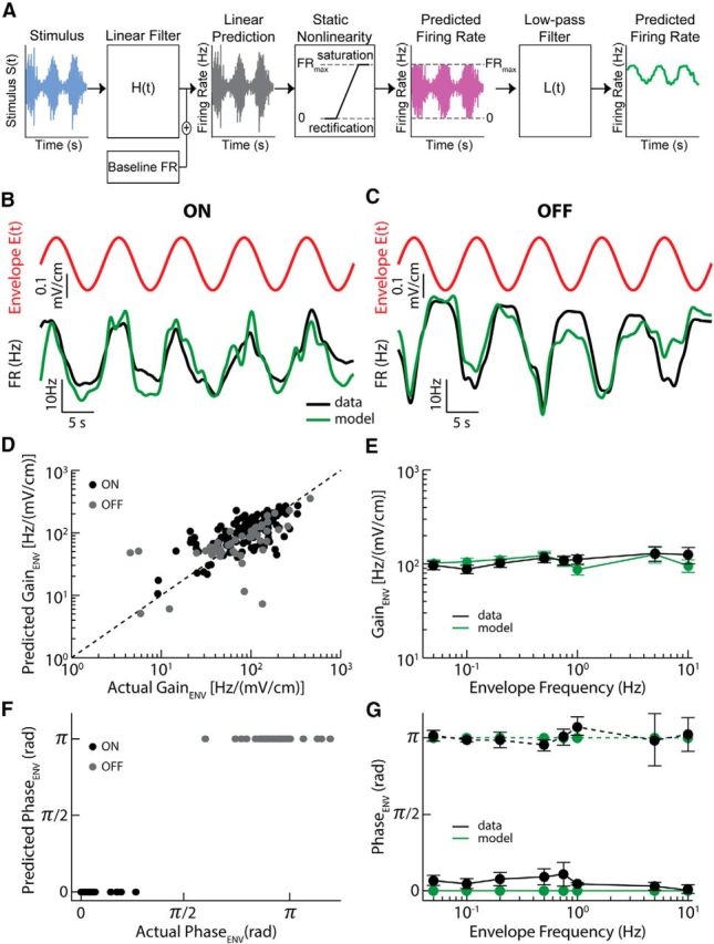
Neural heterogeneities are seen ubiquitously, but how they determine neural response properties remains unclear. Here we show that heterogeneities can either strongly, or not at all, influence neural responses to a given stimulus feature. Specifically, we recorded from peripheral electroreceptor neurons, which display strong heterogeneities in their resting discharge activity, in response to naturalistic stimuli consisting of a fast time-varying waveform (i.e., first-order) whose amplitude (i.e., second-order or envelope) varied slowly in the weakly electric fish Apteronotus leptorhynchus. Although electroreceptors displayed relatively homogeneous responses to first-order stimulus features, further analysis revealed two subpopulations with similar sensitivities that were excited or inhibited by increases in the envelope, respectively, for stimuli whose frequency content spanned the natural range. We further found that a linear-nonlinear cascade model incorporating the known linear response characteristics to first-order features and a static nonlinearity accurately reproduced experimentally observed responses to both first- and second-order features for all stimuli tested. Importantly, this model correctly predicted that the response magnitude is independent of either the stimulus waveform's or the envelope's frequency content. Further analysis of our model led to the surprising prediction that the mean discharge activity can be used to determine whether a given neuron is excited or inhibited by increases in the envelope. This prediction was validated by our experimental data. Thus, our results provide key insight as to how neural heterogeneities can determine response characteristics to some, but not other, behaviorally relevant stimulus features.

Keywords: electroreceptor; envelope; neural heterogeneity; weakly electric fish.

Figure 1.

A. leptorhynchus give behavioral responses to envelopes. A, Schematic of the experimental setup. The animal's electric field is monitored by a pair of electrodes located in front and behind the animal (E1 and E2) while the stimulus is delivered using a separate set of electrodes positioned on each side (gray spheres). The full signal (inset, black) received by the animal was recorded with a dipole ∼2 mm away from the animal (black spheres). Also shown are the frequency contents of the full signal (black), the noisy AM (blue), and the envelope (red). B, Example stimuli showing the stimulus (blue) and its envelope (red) for the two different AM signals used. Left, Frequency range between 5 and 15 Hz, mimicking same sex encounters. Right, Frequency range between 60 and 80 Hz, mimicking opposite sex encounters. Insets, Magnification of the stimulus. C, EOD spectrograms (i.e., EOD power spectrum as a function of time) showing behavioral responses to the stimuli shown in B from an example specimen. D, Population-averaged gain as a function of envelope frequency for the two noisy AM signals used: black represents frequency range 5–15 Hz, n > 10 for each data point; red represents frequency range 60–80 Hz, n > 10 for each data point. E, Population-averaged phase as a function of envelope frequency for the two AM signals used: black represents frequency range 5–15 Hz, n > 10 for each data point; red represents frequency range 60–80 Hz, n > 10 for each data point. Error bars indicate SEM.

Figure 2.

Two classes of peripheral single sensory neurons display ON-type and OFF-type responses to the envelope, respectively. A, Example of an ON-type P-unit responding to an increase in envelope (top) with an increase in firing rate (middle) independently of the AM frequency content: black represents 5–15 Hz; purple represents 60–80 Hz. Bottom, Firing rate response to different envelope frequencies with time normalized to the envelope period. It is seen that the responses mostly superimpose. B, Example of an OFF-type P-unit responding to an increase in envelope (top) with a decrease in firing rate (middle) independently of the AM frequency content: black represents 5–15 Hz; purple represents 60–80 Hz. Bottom, Firing rate response to different envelope frequencies with time normalized to the envelope period. It is seen that the responses mostly superimpose. C, Population-averaged gain to the envelope as a function of envelope frequency for two different AM signals: black represents frequency range 5–15 Hz; purple represents frequency range 60–80 Hz for ON (solid) and OFF (dashed) P-units. D, Population-averaged gain to the envelope as a function of average AM frequency for two different envelope frequencies: black represents 0.05 Hz; purple represents 0.5 Hz for ON (solid) and OFF (dashed) P-units. E, Population-averaged phase to the envelope as a function of envelope frequency for two different AM signals: black represents frequency range 5–15 Hz; purple represents frequency range 60–80 Hz for ON (solid) and OFF (dashed) P-units. F, Population-averaged phase to the envelope as a function of average AM frequency for two different envelope frequencies: black represents 0.05 Hz; purple represents 0.5 Hz for ON (solid) and OFF (dashed) P-units. G, Distributions of gain to the envelope across stimuli for all (dark red), ON (black), and OFF (gray) P-units. There was no significant difference between the gain distributions obtained for ON and OFF P-units (Kolmogorov–Smirnov test, p = 0.34). H, Distributions of phase to the envelope across stimuli for all (dark red), ON (black), and OFF (gray) P-units. The phase distribution for all P-units consists of two well-separated modes (Hartigan's dip test, p ≪ 10⁻³). Further, the phase distributions obtained for ON and OFF P-units were significantly different (Kolmogorov–Smirnov test, p ≪ 10⁻³). Error bars indicate SEM.

Figure 3.

ON-type and OFF-type P-units display similar tuning curves to the stimulus. A, Example of an ON-type P-unit's time-dependent firing rate (bottom) to the stimulus (top). This unit had a baseline firing rate of 270 Hz. The spike train (middle) displays phase-locking as spikes were only elicited in response to the large positive portions of the 60–80 Hz noise stimulus. B, Normalized tuning curve (white dashed line) showing the normalized mean firing rate as well as the density of the firing rate (color plot) as a function of the normalized stimulus for the ON-type P-unit shown in A. C, Example of an OFF-type P-unit's time-dependent firing rate (bottom) to the same stimulus (top) as in A. The spike train (middle) displays phase-locking qualitatively similar to that of the ON-type P-unit shown in A. This unit had a baseline firing rate of 416 Hz. D, Normalized tuning curve (white dashed line) showing the normalized mean firing rate as well as the firing rate density (color plot) as a function of the normalized stimulus for the OFF-type P-unit shown in C. E, Population-averaged gain values with respect to the stimulus for ON-type (black) and OFF type (gray) P-units as a function of the average AM frequency. There were no significant differences between ON- and OFF-type P-units (two-way ANOVA, p > 0.08). Higher-frequency AMs gave rise to higher gain values in general. F, Population-averaged phase values with respect to the stimulus for ON (black) and OFF-type P-units (gray) as function of average AM frequency. There were no significant differences between ON- and OFF-type P-units for any of the AMs used (two-way ANOVA, p > 0.06). Higher-frequency AMs gave rise to higher phase leads in general. Error bars indicate SEM.

Figure 4.

A linear–nonlinear (LN) cascade model predicts P-unit responses to AMs. A, Schematic showing the LN model's structure. The stimulus (left) is first convolved with a filter H(t) that is determined from data to generate the linear predicted firing rate (middle). The baseline firing rate is then added to the linear prediction, and the resulting signal is passed through a static nonlinearity that takes into account rectification and saturation to obtain the predicted firing rate (right). B, Traces showing our model's prediction (bottom, purple) with the actual response (bottom, black) to the AM (top, blue) for an example ON-type P-unit. C, Traces showing the model's prediction (bottom, purple) with the actual response (bottom, black) to the AM (top, blue) for an example OFF-type P-unit. D, Predicted gain to the AM as a function of the actual gain to the AM for all ON-type (black) and OFF-type (gray) P-units in our dataset. The data points are scattered around the identity line (black dashed line). E, Population-averaged gain as a function of the average AM frequency for our data (black) and our model's prediction (green). F, Predicted phase to the AM from our model as a function of actual phase to the AM for all ON-type (black) and OFF-type (gray) P-units in our datasets. G, Population-averaged phase as a function of the average AM frequency for our data (black) and our model's prediction (green). Error bars indicate SEM.

Figure 5.

A linear–nonlinear (LN) cascade model predicts P-unit responses to envelopes. A, Schematic showing the LN model's structure. The stimulus (outside left) is first convolved with a filter H(t) that is determined from data to generate the linear predicted firing rate (left). The baseline firing rate is then added to the linear prediction, and the resulting signal is passed through a static nonlinearity that takes into account rectification and saturation to obtain the predicted firing rate (right). The resulting signal is then low-pass filtered to obtain the predicted response to the envelope (outside right). B, Traces showing our model's prediction (bottom, green) with the actual response (bottom, black) to the envelope (top, red) for an example ON-type P-unit. C, Traces showing the model's prediction (bottom, green) with the actual response (bottom, black) to the envelope (top, red) for an example OFF-type P-unit. D, Predicted gain to the envelope as a function of the actual gain to the envelope for all ON-type (black) and OFF-type (gray) P-units in our dataset. The data points are scattered around the identity line (dashed black line). E, Population-averaged gain as a function of envelope frequency for our data (black) and our model's prediction (green). F, Predicted phase to the envelope from our model as a function of actual phase to the envelope for all ON-type (black) and OFF-type (gray) P-units in our dataset. G, Population-averaged phase as a function of envelope frequency for our data (black) and our model's prediction (green) for ON (bottom) and OFF (top) -type P-units. Error bars indicate SEM.

Figure 6.

Model predicts baseline firing determines ON- vs OFF-type responses to envelopes. A, Left, Schematic showing why a P-unit with low baseline firing rate gives an ON-type response (bottom, solid purple curve) to the envelope of a sinusoidal stimulus (top): because of rectification at zero, the mean firing rate increases (bottom, solid horizontal purple line) during stimulation compared with what it would be if no rectification occurred (dashed horizontal black line) as indicated by the arrow. Bottom, Dashed black curve indicates the response to the same stimulus without the static nonlinearity. Middle, Schematic showing why a P-unit with baseline firing rate in the middle of the dynamic range (i.e., equal to FR_max/2) does not respond to the envelope. For this unit, the increase in firing rate due to rectification is exactly compensated by the decrease due to saturation (bottom, solid green curve). Thus, the mean firing rate (bottom, horizontal solid green line) is not different from the baseline firing rate (bottom, horizontal dashed black line). Bottom, Dashed black curve indicates the response to the same stimulus without the static nonlinearity. Right, Schematic showing why a P-unit with high baseline firing rate gives an OFF-type response (bottom, solid blue curve) to the envelope of a sinusoidal stimulus (top): because of saturation, the mean firing rate decreases (bottom, blue horizontal line) during stimulation compared with what it would be if no saturation occurred (dashed black horizontal line) as indicated by the arrow. Bottom, Dashed black curve indicates the response to the same stimulus without the static nonlinearity. B, The gain displays a minimum when the normalized baseline firing rate (i.e., the baseline firing rate divided by the maximum firing rate obtained during stimulation) is equal to 0.5. C, Phase of the response as a function of normalized baseline firing rate. Responses are ON-type for normalized baseline firing rates <0.5 and OFF-type otherwise.

Figure 7.

Verifying modeling predictions. A, Population-averaged gain values for P-units with low (<0.48, N = 72), medium (>0.48 and <0.52, N = 15), and high (>0.52, N = 49) normalized baseline firing rates. P-units with low and high normalized baseline firing rates displayed significantly larger gains than P-units with medium normalized baseline firing rates (two-way ANOVA, p < 0.004). B, ON-type (black) responses are observed preferentially for P-units with a normalized baseline firing rate <0.5, whereas OFF-type (gray) responses are instead preferentially observed for P-units with higher normalized baseline firing rates. C, The normalized baseline firing rate of ON-type P-units was on average (0.38 ± 0.01) significantly less than 0.5 (t test, n_ON = 72, p ≪ 10⁻³), whereas that of OFF-type P-units was on average (0.57 ± 0.01) significantly greater than 0.5 (t test, n_OFF = 49, p ≪ 10⁻³). Horizontal dashed line indicates the threshold value of 0.5.

Figure 8.

The P-unit population transmits detailed information about the envelope independently of envelope frequency. A, Schematic of the stimulus reconstruction procedure. Each neural response R_i(t) to the signal E(t) (left) was convolved (⊗) with an optimal filter K_i(t) (middle). The results were then summed to get the estimated signal E_est(t) (right). B, Coding fraction (i.e., the fraction of the envelope that is successfully reconstructed) as a function of population size for all envelope frequencies using a 5–15 Hz AM stimulus. For comparison, the coding fraction quantifying the fraction of the unmodulated 5–15 Hz AM stimulus that is correctly reconstructed is also shown. Similar results were obtained using a 60–80 Hz AM stimulus (data not shown). C, Population-averaged coding fraction (i.e., the fraction of the envelope that is successfully reconstructed) as a function of population size for ON-type P-units (black), OFF-type P-units (gray), and a mixed population of ON + OFF-type P-units (dark red, 50% ON and 50% OFF). The coding fraction for mixed population is significantly greater than that obtained when considering either ON- or OFF-type P-units for population ≥5. *p = 0.01 (two-way ANOVA with Bonferroni post hoc correction). D, Population-averaged coding fraction for the envelope as a function of the average AM frequency for two envelope frequencies: dark blue represents 0.05 Hz; light blue represents 0.5 Hz. The coding fraction increased as a function of AM frequency and both curves were not significantly different from one another (t test, p = 0.7492). E, Population-averaged coding fraction obtained for the envelope as a function of envelope frequency for 5–15 Hz (open circles) and 60–80 Hz (filled circles) using a mixed population of n = 6 P-units.

References

1. Avila-Åkerberg O, Krahe R, Chacron MJ. Neural heterogeneities and stimulus properties affect burst coding in vivo. Neuroscience. 2010;168:300–313. doi: 10.1016/j.neuroscience.2010.03.012. - DOI - PMC - PubMed
1. Baker CL., Jr Central neural mechanisms for detecting second-order motion. Curr Opin Neurobiol. 1999;9:461–466. doi: 10.1016/S0959-4388(99)80069-5. - DOI - PubMed
1. Bannister NJ, Larkman AU. Dendritic morphology of CA1 pyramidal neurones from the rat hippocampus: II. Spine distributions. J Comp Neurol. 1995a;360:161–171. doi: 10.1002/cne.903600112. - DOI - PubMed
1. Bannister NJ, Larkman AU. Dendritic morphology of CA1 pyramidal neurones from the rat hippocampus: I. Branching patterns. J Comp Neurol. 1995b;360:150–160. doi: 10.1002/cne.903600111. - DOI - PubMed
1. Bastian J. Electrolocation II: the effects of moving objects and other electrical stimuli on the activities of two categories of posterior lateral line lobe cells in Apteronotus albifrons. J Comp Physiol A. 1981;144:481–494. doi: 10.1007/BF01326833. - DOI
Publication types
LinkOut - more resources