Covariance Matrix Estimation for the Cryo-EM Heterogeneity Problem

Abstract

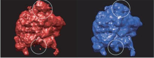
In cryo-electron microscopy (cryo-EM), a microscope generates a top view of a sample of randomly oriented copies of a molecule. The problem of single particle reconstruction (SPR) from cryo-EM is to use the resulting set of noisy two-dimensional projection images taken at unknown directions to reconstruct the three-dimensional (3D) structure of the molecule. In some situations, the molecule under examination exhibits structural variability, which poses a fundamental challenge in SPR. The heterogeneity problem is the task of mapping the space of conformational states of a molecule. It has been previously suggested that the leading eigenvectors of the covariance matrix of the 3D molecules can be used to solve the heterogeneity problem. Estimating the covariance matrix is challenging, since only projections of the molecules are observed, but not the molecules themselves. In this paper, we formulate a general problem of covariance estimation from noisy projections of samples. This problem has intimate connections with matrix completion problems and high-dimensional principal component analysis. We propose an estimator and prove its consistency. When there are finitely many heterogeneity classes, the spectrum of the estimated covariance matrix reveals the number of classes. The estimator can be found as the solution to a certain linear system. In the cryo-EM case, the linear operator to be inverted, which we term the projection covariance transform, is an important object in covariance estimation for tomographic problems involving structural variation. Inverting it involves applying a filter akin to the ramp filter in tomography. We design a basis in which this linear operator is sparse and thus can be tractably inverted despite its large size. We demonstrate via numerical experiments on synthetic datasets the robustness of our algorithm to high levels of noise.

Keywords: Fourier projection slice theorem; X-ray transform; classification; covariance matrix estimation; cryo-electron microscopy; heterogeneity; high-dimensional statistics; inverse problems; principal component analysis; spherical harmonics; structural variability.

Figure 1

Classical (left) and hybrid (right) states of 70S E. Coli ribosome (image source: [29]).

Figure 2

Illustrations of high-dimensional PCA

Figure 3

The triangular area filter. ξ1 induces a strip on S2 of width proportional to 1/|ξ1 ^{| (blue); ξ}2 ^{induces a strip of width proportional to 1/|ξ}2 | (red). The strips intersect in two parallelogram-shaped regions (white), each with area proportional to 1/|ξ1 ^{× ξ}2^{|. Hence, K(ξ}1 ^{, ξ}2) is inversely proportional to the area of the triangle spanned by ξ1^{, ξ}2 (cyan).

Figure 4

The even basis functions up to f14 (r). Note that they become less oscillatory as k increases, and that f^k (r) ~ r^k at the origin. The odd basis functions have a similar structure and so are not pictured.

Figure 5

Block diagonal structure of PPs. The shaded rectangles represent the nonzero entries. For an explanation of the specific pairing of angular and radial functions, see (5.27) and (5.19) and the preceding discussion. A short calculation shows that the kth block of PĈs has size $(k+1)\times \frac{(k+1)(k+2)}{2}$.

Figure 6

The smallest and largest eigenvalues of (the continuous version of ) LPk,k, for 0 ≤ k ≤ 15. The smallest eigenvalues approach their theoretical lower bound of 1/2π as k increases. The largest eigenvalues show a clear linear dependence on k.

Figure 7

This figure depicts the effect of mean subtraction on projection images in the context of a two-class heterogeneity. The bottom row projections are obtained from the top row by mean subtraction. Columns (a) and (b) are clean projection images of the two classes from a fixed viewing angle. Columns (c) and (d) are both noisy versions of column (a). The image in the top row of column (c) has an SNR of 0.96, but the SNR of the corresponding mean-subtracted image is only 0.05. In column (d), the top image has an SNR of 0.19, but the mean-subtracted image has SNR 0.01. Note: the SNR values here are not normalized by N ² /N ² in order to illustrate the signal present in a projection image.

Figure 8

Cross-sections of reconstructions of the mean, top eigenvector, and two volumes for three different SNR values. The top row is clean, the second row corresponds to SNR_het = 0.013 (0.25), the third row to SNR_het = 0.003 (0.056), and the last row to SNR_het = 0.0013 (0.025). (a) SNR_het = 0.013(0.25) (b) SNR_het = 0.003(0.056) (c) SNR_het = 0.0013(0.025)

Figure 9

Eigenvalue histograms of ΣP n xin the two-volume case for three SNR values. Note that as the SNR decreases, the distribution of eigenvalues associated with noise comes increasingly closer to the top eigenvalue that corresponds to the structural variability, and eventually the latter is no longer distinguishable.

Figure 10

FSC curves for the mean volume, top eigenvector, and one mean-subtracted volume at the same three SNRs as in Figure 8. Note that the mean volume is reconstructed successfully for all three SNR levels. On the other hand, the top eigenvector and volume are recovered at the highest two SNR levels but not at the lowest SNR.

Figure 11

Correlations of computed quantities with their true values for different SNRs (averaged over 10 experiments) for the two-volume case. Note that in the two-volume case, the mean-subtracted volume correlations are essentially the same as the eigenvector correlation (the only small discrepancy is that we subtract the true mean rather than the computed mean to obtain the former).

Figure 12

Histograms of αs for two-class case. Note that (a) has a bimodal distribution corresponding to two heterogeneity classes, but these two distributions merge as SNR decreases. (0.002) and 0.003 (0.006). Note that this behavior is tied to the spectral gap (separation of top eigenvalues from the bulk) of Σ^{P n}. Indeed, the disappearance of the spectral gap going from panel (b) to panel (c) of Figure 9 coincides with the estimated top eigenvector becoming uncorrelated with the truth, as reflected in Figures 10(b) and 11(a). This phase transition behavior is very similar to that observed in the usual high-dimensional PCA setup, described in section 2.3.

Figure 13

Cross sections of clean and reconstructed objects for the three-class experiment. The top row is clean, the second row corresponds to SNR_het = 0.044 (0.3), the third row to SNR_het = 0.0044 (0.03), and the last row to SNR_het = 0.0015 (0.01).

Figure 14

Eigenvalue histograms of reconstructed covariance matrix in the three-class case for three SNR values. Note that the noise distribution initially engulfs the second eigenvalue, and eventually the top eigenvalue as well.

Figure 15

FSC curves for the mean volume, top eigenvector, and one mean-subtracted volume at the same three SNRs as in Figure 13. Note that the mean volume is reconstructed successfully for all three SNR levels, and that the second eigenvector is recovered less accurately than the first.

Figure 16

Correlations of computed means, eigenvectors, and mean-subtracted volumes with their true values for different SNRs (averaged over 30 experiments). Note that the mean volume is consistently recovered well, whereas recovery of the eigenvectors and volumes exhibits a phase-transition behavior.

Figure 17

The coordinates αs for the three-class case, colored according to true class. The middle scatter plot is near the transition at which the three clusters coalesce.

Figure 18

Eigenvalue histograms of covariance matrix reconstructed in continuous variation case.

Figure 19

Scatter plots (with some outliers removed) of αs for high SNR values.

References

1. Amunts A, Brown A, Bai X, Llaácer J, Hussain T, Emsley P, Long F, Murshudov G, Scheres S, Ramakrishnan V. Structure of the yeast mitochondrial large ribosomal subunit. Science. 2014;343:1485–1489. - PMC - PubMed
1. Baddour N. Operational and convolution properties of three dimensional Fourier transforms in spherical polar coordinates. J. Opt. Soc. Amer. A. 2010;27:2144–2155. - PubMed
1. Bai X, Fernandez I, McMullan G, Scheres S. Ribosome structures to near-atomic resolution from thirty thousand cryo-em particles. eLife. 2013;2:e00461. - PMC - PubMed
1. Baik J, Ben Arous G, Páecháe S. Phase transition of the largest eigenvalue for nonnull complex sample covariance matrices. Ann. Probab. 2005;33:1643–1697.
1. Baik J, Silverstein JW. Eigenvalues of large sample covariance matrices of spiked population models. J. Multivariate Anal. 2006;97:1382–1408.
LinkOut - more resources