. 2015 May;22(1):1-20.
doi: 10.1016/j.media.2015.01.005. Epub 2015 Feb 3.

A novel cortical thickness estimation method based on volumetric Laplace-Beltrami operator and heat kernel

Affiliations

A novel cortical thickness estimation method based on volumetric Laplace-Beltrami operator and heat kernel

Gang Wang et al. Med Image Anal. 2015 May.

Abstract

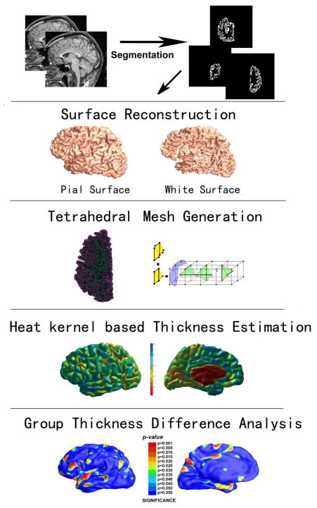
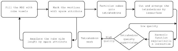
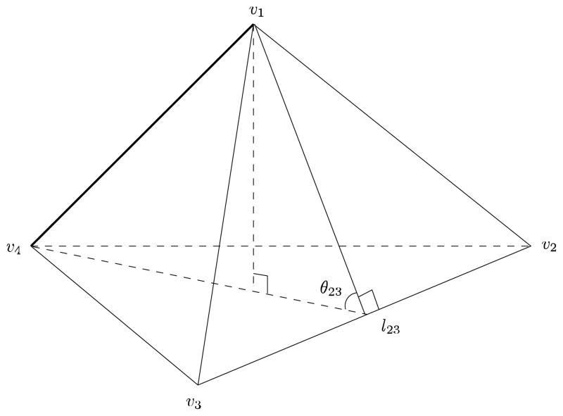
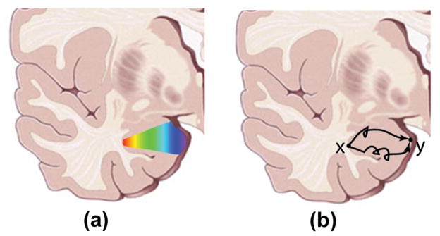
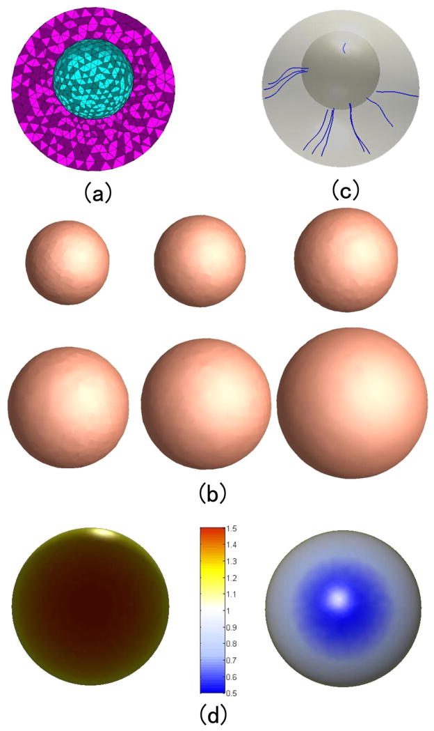
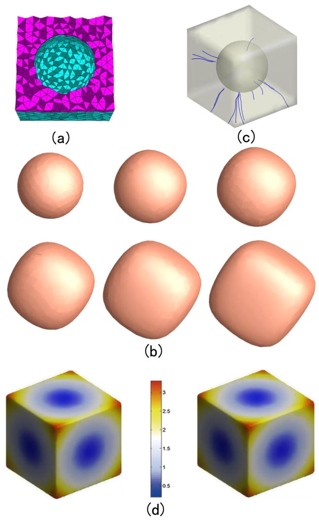
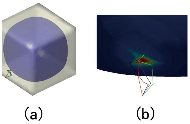
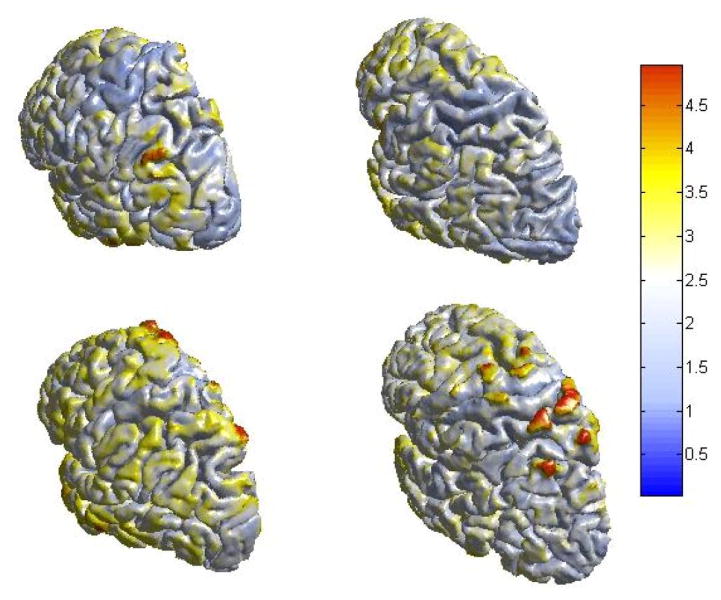
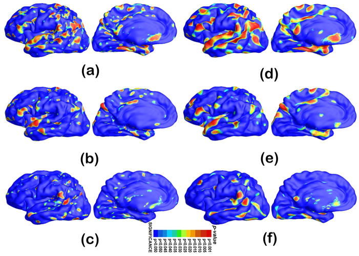
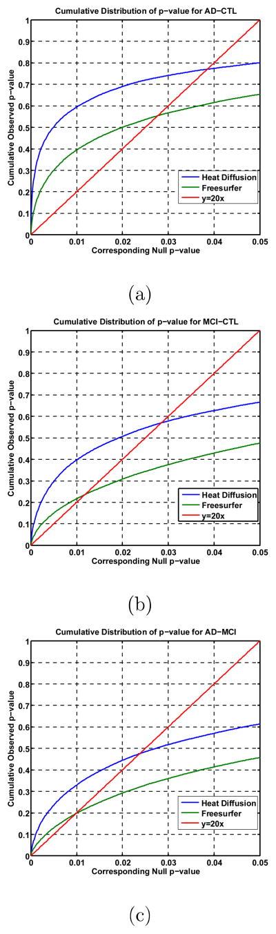
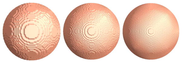
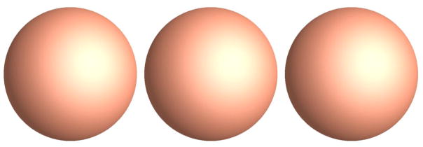
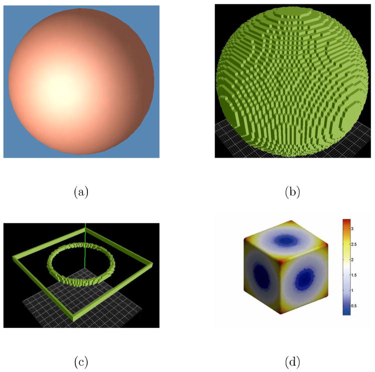
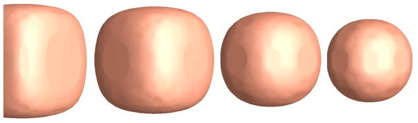
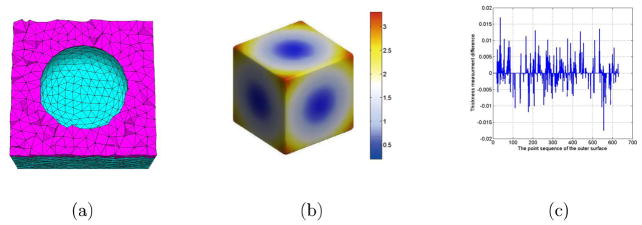
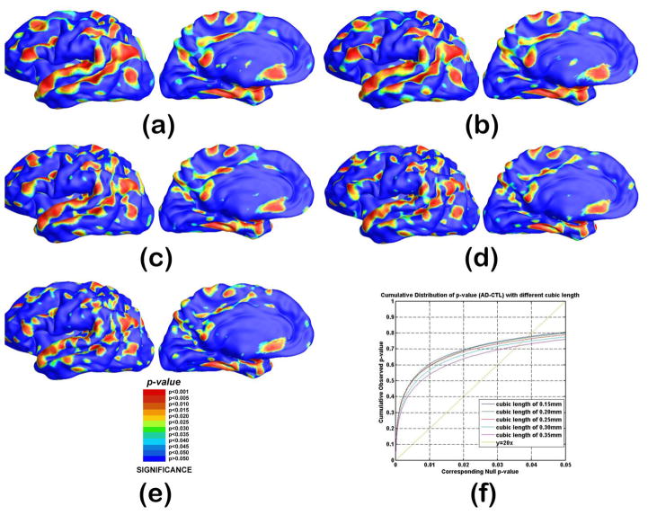
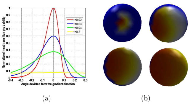
Cortical thickness estimation in magnetic resonance imaging (MRI) is an important technique for research on brain development and neurodegenerative diseases. This paper presents a heat kernel based cortical thickness estimation algorithm, which is driven by the graph spectrum and the heat kernel theory, to capture the gray matter geometry information from the in vivo brain magnetic resonance (MR) images. First, we construct a tetrahedral mesh that matches the MR images and reflects the inherent geometric characteristics. Second, the harmonic field is computed by the volumetric Laplace-Beltrami operator and the direction of the steamline is obtained by tracing the maximum heat transfer probability based on the heat kernel diffusion. Thereby we can calculate the cortical thickness information between the point on the pial and white matter surfaces. The new method relies on intrinsic brain geometry structure and the computation is robust and accurate. To validate our algorithm, we apply it to study the thickness differences associated with Alzheimer's disease (AD) and mild cognitive impairment (MCI) on the Alzheimer's Disease Neuroimaging Initiative (ADNI) dataset. Our preliminary experimental results on 151 subjects (51 AD, 45 MCI, 55 controls) show that the new algorithm may successfully detect statistically significant difference among patients of AD, MCI and healthy control subjects. Our computational framework is efficient and very general. It has the potential to be used for thickness estimation on any biological structures with clearly defined inner and outer surfaces.

Keywords: Cortical thickness; False discovery rate; Heat kernel; Spectral analysis; Tetrahedral mesh.


Figures

Figure 1
Figure 1
Algorithm pipeline illustrated by the intermediate results.
Figure 2
Figure 2
Tetrahedral mesh generation work flow.
Figure 3
Figure 3
Two examples of generated tetrahedral meshes with the different resolutions and their tetrahedral element qualities.
Figure 4
Figure 4
Illustration of half-edge structure for surface representation (a) and the proposed half-face structure for tetrahedron representation (b). (a) was obtained from (MakeHuman Project Team, 2013).
Figure 5
Figure 5
Illustration of a tetrahedron. By convention, we say that the edge [v1, v4] is against [v2, v3] and the dihedral angle, θ23, in this tetrahedron. l23 is the length of edge [v2, v3]. This relationship is used to define volumetric Laplace-Beltrami operator.
Figure 6
Figure 6
Illustration of heat diffusion on cortical structure. Two boundaries are examples of pial and white matter surfaces. (a) Heat diffusion illustration with spectrum; (b) diffusion distance illustrated as random walk. Our heat kernel method may be able to capture the subtle difference determined by the intrinsic geometry structures because it estimates the heat transition probability on every intermediate point such that it may capture more regional information than other harmonic function methods (e.g. Jones et al., 2000).
Figure 7
Figure 7
The isothermal surfaces, streamline and thickness computation between the outer spherical surface to the inner spherical surface. (a) is the volumetric mesh. (b) shows the different isothermal surfaces. (c) shows some computed streamlines between two surfaces. (d) shows the color map of the computed thickness values.
Figure 8
Figure 8
The isothermal surfaces, streamline and thickness computation between the outer cubic surface to the inner spherical surface. (a) is the volumetric mesh. (b) shows the different isothermal surfaces. (c) shows some computed streamlines between two surfaces. (d) shows the color map of the computed thickness values.
Figure 9
Figure 9
The heat transition paths from the specific point on the outer isothermal surface (temperature 1°) to the different points on the inner isothermal surface (temperature 0.91°). (a) shows the heat transition paths of the different transition probabilities and (b) shows the enlarged interval paths between the two isothermal surfaces.
Figure 10
Figure 10
Four cortical thickness measurement results. The values of thickness (mm) increase as the color goes from blue to yellow and to red.
Figure 11
Figure 11
Statistical p-map results with the thickness measures of heat kernel diffusion and FreeSurfer on surface templates show group differences among three different groups of AD subjects (N = 51), MCI subjects (N = 45) and control subjects (N = 55). (d–f) are the results of our method, (a–c) are results of FreeSurfer method. (a) and (d) are group difference results of AD vs. control. (b) and (e) are group difference results of control vs. MCI. (c) and (f) are group difference results of MCI vs.AD. Non-blue colors show vertices with statistical differences, uncorrected. The q-values for these maps are shown in Table 2. The q-value is the highest threshold that can be applied to the statistical map while keeping the false discovery rate below 5%. (For interpretation of the references to colour in this figure legend, the reader is referred to the web version of this article.)
Figure 12
Figure 12
The cumulative distributions of p-values comparison for difference detected between three groups (AD, MCI, CTL). The color-coded p-maps are shown in Fig. 11. and their q-values are shown in Table 2. In the CDF, the q-values are the intersection point of the curve and the y = 20x line. In a total of 3 comparisons, the heat diffusion method achieved the highest q-values.
Figure 13
Figure 13
The boundaries extracted from the cubic meshes with the different cube sizes.
Figure 14
Figure 14
The boundaries extracted from the tetrahedral meshes with the different resolutions.
Figure 15
Figure 15
The constructed 3D volumetric grid mesh from the inner boundary of Fig. 8(a). Fig. 15(a) shows the spherical boundary and (b) shows the generated 3D voxel grid mesh of Fig. 15(a). (c) shows a slice of the total boundaries of the 3D volumetric grid mesh. And (d) shows the color map of the computed thickness values based on the finite difference method.
Figure 16
Figure 16
The isothermal surfaces of 0.8°, 0.7°, 0.5° and 0.4° are shown from left to right.
Figure 17
Figure 17
The thickness measurement comparison between the different tetrahedral resolution. (a) is the reconstructed tetrahedral mesh with higher resolution, (b) is the thickness measurement result, and (c) is the thickness differences between the two surface of the different resolution.
Figure 18
Figure 18
Statistical p-map results with the heat diffusion thickness measures of different cubic edge length on surface templates representing group differences among two different groups (AD-CTL), of AD subjects (N=51) and control subjects (N=55). Non-blue colors show vertices with statistical differences, uncorrected, (a)–(e) are the results of cubic edge length of 0.15, 0.20, 0.25, 0.30 and 0.35mm on group difference between AD and control, respectively. The cumulative distributions of p-values comparison for difference detected between AD and CTL are shown in (f). The q-values for these maps are shown in Table 3.
Figure 19
Figure 19
Influence effect of heat transfer time interval. (a) shows the relationships between normalized heat transfer probabilities from the specific point on the higher temperature isosurface (0.95°) to the points on the lower temperature (0.90°) and the angle deviates from the gradient direction. The curves with different colors represent the different heat transfer time intervals. (b) shows the heat acceptance results on the lower temperature isosurface with the different time interval. The top left and right are the time interval of 0.02 and 0.03, the bottom left and right are the time interval of 0.04 and 0.2.

Similar articles

Cited by

References

    1. Adamson CL, Wood AG, Chen J, Barton S, Reutens DC, Pantelis C, Velakoulis D, Walterfang M. Thickness profile generation for the corpus callosum using Laplace’s equation. Hum Brain Mapp. 2011;32:2131–2140. - PMC - PubMed
    1. Alzheimer’s Association. Alzheimer’s disease facts and figures. Alzheimer’s Association; 2012. http://www.alz.org. - PubMed
    1. Benjamini Y, Hochberg Y. Controlling the False Discovery Rate: A Practical and Powerful Approach to Multiple Testing. Journal of the Royal Statistical Society Series B (Methodological) 1995;57:289–300.
    1. Berg L. Clinical Dementia Rating (CDR) Psychopharmacol Bull. 1988;24:637–639. - PubMed
    1. Braak H, Braak E. Neuropathological stageing of Alzheimer-related changes. Acta Neuropathol. 1991;82:239–259. - PubMed

Publication types