An ensemble-averaged, cell density-based digital model of zebrafish embryo development derived from light-sheet microscopy data with single-cell resolution

Abstract

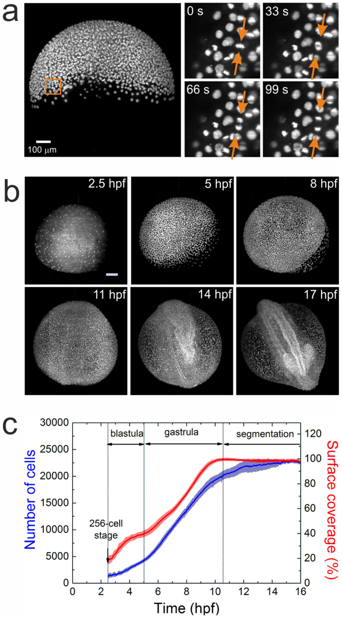
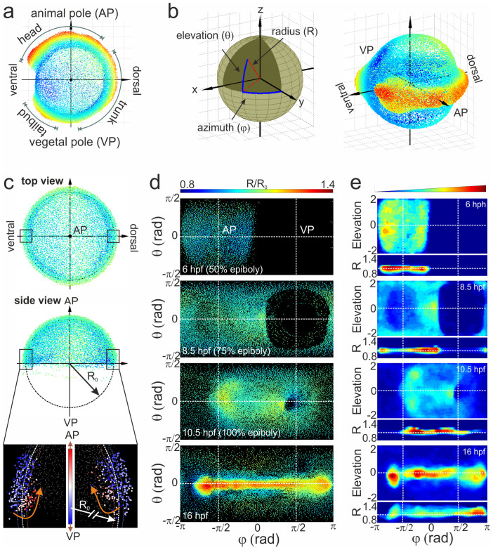
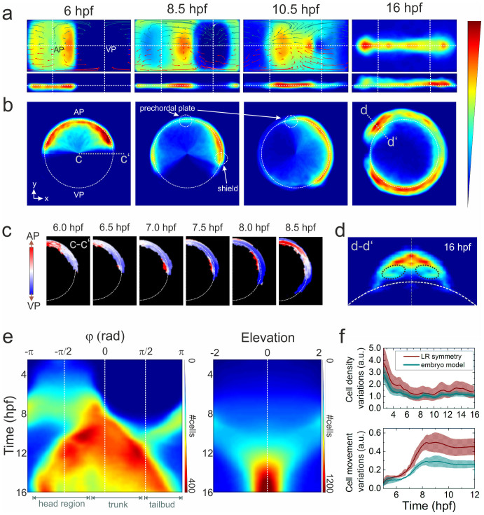
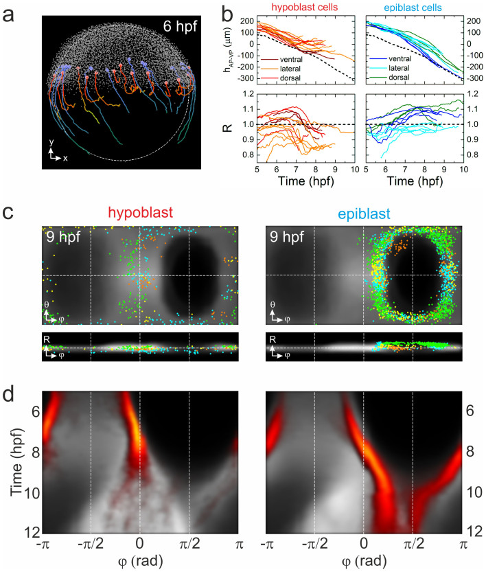
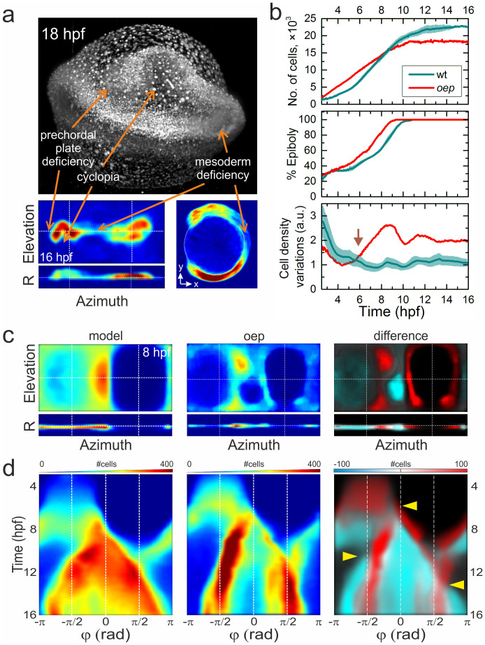
A new era in developmental biology has been ushered in by recent advances in the quantitative imaging of all-cell morphogenesis in living organisms. Here we have developed a light-sheet fluorescence microscopy-based framework with single-cell resolution for identification and characterization of subtle phenotypical changes of millimeter-sized organisms. Such a comparative study requires analyses of entire ensembles to be able to distinguish sample-to-sample variations from definitive phenotypical changes. We present a kinetic digital model of zebrafish embryos up to 16 h of development. The model is based on the precise overlay and averaging of data taken on multiple individuals and describes the cell density and its migration direction at every point in time. Quantitative metrics for multi-sample comparative studies have been introduced to analyze developmental variations within the ensemble. The digital model may serve as a canvas on which the behavior of cellular subpopulations can be studied. As an example, we have investigated cellular rearrangements during germ layer formation at the onset of gastrulation. A comparison of the one-eyed pinhead (oep) mutant with the digital model of the wild-type embryo reveals its abnormal development at the onset of gastrulation, many hours before changes are obvious to the eye.

Figure 1. Imaging and quantification of embryo development.

(a) MIP image of an embryo at 50% epiboly; a sequence of four time-lapse images from a selected region (square) is shown on the right. The arrows point to a dividing cell. (b) Typical maximum intensity projection images of a zebrafish embryo at 2.5, 5, 8, 11, 14, and 17 hpf. Scale bar is 100 μm. (c) Time dependence of the average cell number and yolk surface coverage during embryo development, computed from an ensemble of five embryos.

Figure 2. Alignment of cell coordinates according to the standard embryo position.

(a) Standard embryo representation on the yolk sphere at later developmental time points (16 hpf); the color code denotes the distance from the origin. (b) Transformation from Cartesian to spherical coordinates. For the cylindrical projection, the anterior-posterior embryo axis was placed at zero elevation (equator); by setting the dorsal embryo side at zero azimuths, the animal (AP) and vegetal (VP) poles appeared at the −π/2 and π/2 azimuthal angles, respectively. (c) Embryo alignment at the early gastrula stage. Top and side views show the symmetrically distribution of cells around the AP. The color code denotes the distance from the origin as in (a). The radius of the embryo sphere R₀ is determined according to the border between hypoblast and epiblast cell layers (lower panel of the side view; the color code denotes the movement direction) which display opposite movement at 7 hpf towards the AP (red) and VP (blue), respectively. (d) Spherical projection of cell nuclei coordinates from a single embryo on a 2D map using azimuthal and elevation angles. Typical 2D maps of cell nuclei coordinates are plotted at 6, 8.5, 10.5 and 16 hpf using the equidistant cylindrical projection. The radial coordinate is color-coded in the range between 0.8 and 1.4. (e) 2D maps of integrated cell nuclei density from a single sample using the area-preserving Gall-Peters (2 sinθ versus φ) and R versus φ projection of the same datasets as in (d). The blue-to-red color code denotes the increase of the normalized cell density in arbitrary units.

Figure 3. Ensemble-averaged digital model.

(a) Averaged cell density cylindrical projections in spherical coordinates (azimuth vs. elevation). The vector fields represent 2 h collective cell migration patterns, computed by locally averaging the displacement of cells with R < 1 (red arrows) and R > 1 (dark cyan). For symmetry reasons, only half of each vector field is shown. (b) Planar projections in Cartesian coordinates at selected times; the dashed white line indicates the embryo sphere, and the blue-to-red color code represents the normalized cell density (in arbitrary units). (c) Projection of cell density movement at the embryo dorsal side from 6 to 8.5 hpf; the direction is encoded by color (toward the AP: red, toward the VP: blue). (d) Cell density projection at 16 hpf at a cross-section through the head region (d–d′) depicted in panel (b); the dashed black lines mark the eye positions. The color code is the same as in (a) and (b). (e) Kymographs of azimuthal (left panel) and elevation (right panel) cell density projections; the color code denotes the number of cells per azimuthal or elevation segment, respectively. (f) Quantitative analysis of cell density (upper panel) and movement (lower panel) variations with respect to the midline mirror (left-right) symmetry (within each sample) and to the model. The solid lines represent averages over the ensemble; the shaded regions around the lines depict the ±σ values of statistical significance that include sample heterogeneity as well as statistical errors due to cell number variations within voxels (σ² = (σ_samples)² + (〈σ_ΔN〉)²).

Figure 4. Visualization of blastoderm margin development.

(a) Lateral view of a zebrafish embryo at 6 hpf; cells are shown as small gray dots. The colored spheres denote examples of hypoblast (red) and epiblast (blue) cells; also shown are their trajectories from 6–10 hpf. (b) Typical trajectories of selected hypoblast (left) and epiblast (right) cells during gastrulation; represented by their positions projected onto the AP-VP axis (top) and their radial positions (bottom). Trajectories are color-coded according to dorsal, lateral or ventral position; the dashed line (upper graphs) represents the position of the blastoderm margin. (c) Gall-Peters projections and radial plots of cell positions, showing an overlay of hypoblast (left) and epiblast (right) cells from different samples (shown in different colors) on top of the averaged model cell density (gray) at 9 hpf. (d) Hypoblast (left) and epiblast (right) azimuthal cell density kymographs (yellow/red) overlayed onto the digital model kymograph from Fig. 3e (gray).

Figure 5. Morphological changes of an oep mutant.

(a) MIP image of an oep mutant embryo at 18 hpf and cell density projection at 16 hpf. Arrows indicate characteristic phenotypical oep features. (b) Quantitative comparison of wt and oep mutant cell number (top), epiboly (middle), and cell density variation during development (bottom). Data of the wt embryo (Fig. 3F and Supplementary Fig. 3) are included for comparison. (c) Left and middle panels: Cell density projections at 8 hpf of the averaged model and the individual oep mutant, respectively, depicted in the same color code as in Fig. 3a. Right panel: Overlay of differences (negative: cyan, positive: red) in cell densities between the mutant and the wt model on top of the model data (gray). (d) Kymographs of azimuthal projections, panels arranged as in (c). Arrows point to pronounced developmental differences between the oep mutant and the wt embryo model.

References

1. Howe K. et al. The zebrafish reference genome sequence and its relationship to the human genome. Nature 496, 498–503 (2013). - PMC - PubMed
1. Kettleborough R. N. et al. A systematic genome-wide analysis of zebrafish protein-coding gene function. Nature 496, 494–497 (2013). - PMC - PubMed
1. Blackburn P. R., Campbell J. M., Clark K. J. & Ekker S. C. The CRISPR system--keeping zebrafish gene targeting fresh. Zebrafish 10, 116–118 (2013). - PMC - PubMed
1. Baskin J. M., Dehnert K. W., Laughlin S. T., Amacher S. L. & Bertozzi C. R. Visualizing enveloping layer glycans during zebrafish early embryogenesis. Proc. Natl Acad. Sci. USA. 107, 10360–10365 (2010). - PMC - PubMed
1. Keller P. J., Schmidt A. D., Wittbrodt J. & Stelzer E. H. Reconstruction of zebrafish early embryonic development by scanned light sheet microscopy. Science 322, 1065–1069 (2008). - PubMed
Publication types
LinkOut - more resources