doi: 10.1021/cr500501m.
Epub 2015 Mar 9.
The mesosphere and metals: chemistry and changes
Affiliations
- PMID: 25751779
- PMCID: PMC4448204
- DOI: 10.1021/cr500501m
Item in Clipboard
The mesosphere and metals: chemistry and changes
Chem Rev.
.
No abstract available
Figures

Temperature (K) as a
function of latitude and height in the MLT
for January (left panel) and July (right panel) (averaged from 2004
to 2011). Also plotted are wind vectors (m s–1)
which combine the meridional wind v with the vertical
wind w (×500). Output from the Whole Atmosphere
Community Climate Model.

Energy balance
in the MLT: roughly equal inputs of energy from
absorption of solar energy by O2 and O3 and
breaking gravity waves are balanced by radiative loss principally
through 15 μm emission of CO2.

Zonally averaged temperature (K) at 87 km as a function of latitude
and month. Output from the Whole Atmosphere Community Climate Model.

Diurnal variation as
a function of the height of the (a) O density
(1010 atom cm–3), (b) H density (107 atom cm–3), and (c) O3 density
(109 molecules cm–3) for October at Kühlungsborn,
Germany (54° N, 12° E) (averaged from 2004 to 2011). Output
from the Whole Atmosphere Community Climate Model.

Atomic O measurements made by rocket-borne resonance fluorescence
instruments during summer in Northern Sweden (67.9° N). Adapted
with permission from ref (10). Copyright 2005 Copernicus Publications on behalf of the
European Geosciences Union.

Seasonal variation as a function of the height of the
zonally averaged
(a) NO density (108 molecules cm–3),
(b) H2O density (107 molecules cm–3), and (c) H density (107 atom cm–3)
at 54° N (averaged from 2004 to 2011). Output from the Whole
Atmosphere Community Climate Model.
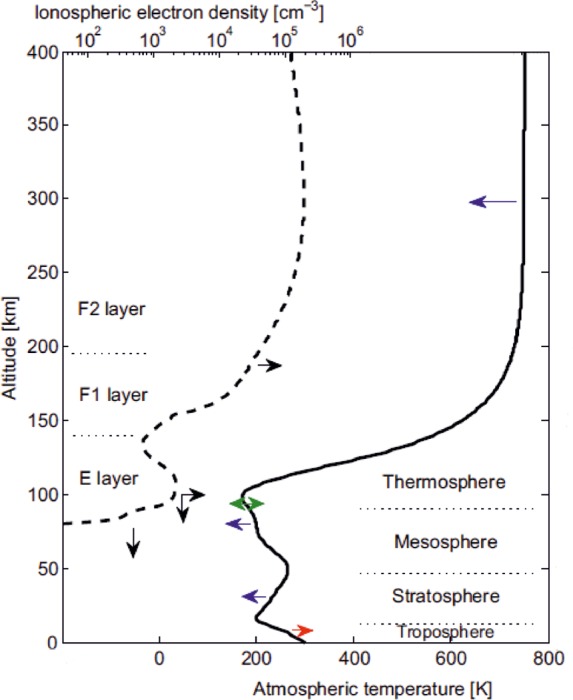
Structure and trends in the Earth’s atmosphere. The atmospheric
layers on the right are defined by the temperature profile (solid
line, bottom abscissa). The ionospheric layers on the left are defined
by the electron density profile (broken line, top abscissa). Arrows
denote the direction of observed changes in the past 3–4 decades:
red, warming; blue, cooling; green, no overall temperature change;
black, changes in the maximum electron density (horizontal) and the
height of ionospheric layers (vertical). Adapted with permission from
ref (22). Copyright
2006 American Association for the Advancement of Science.

Annual mean long-term temperature trends (K decade–1) in the mesosphere over the tropical latitudes. The
rocketsonde
trends of the 1970s and 1980s are compared with the trend obtained
during the past two decades using satellite and lidar data (see the
text for further details). The horizontal line shading represents
roughly the range of trends as revealed during the past two decades.
Reprinted with permission from ref (21). Copyright 2011 John Wiley & Sons, Inc.

Comparison of the seasonal
PMC frequency of occurrence measured
by SBUV radiometers by latitude band and the fit to a linear regression
in time and solar activity. The error bars are the confidence limits
in the individual seasonal mean values based on counting statistics,
which do not reflect other factors such as interannual variability
in large-scale dynamics. Reprinted with permission from ref (76). Copyright 2009 John Wiley
& Sons, Inc.
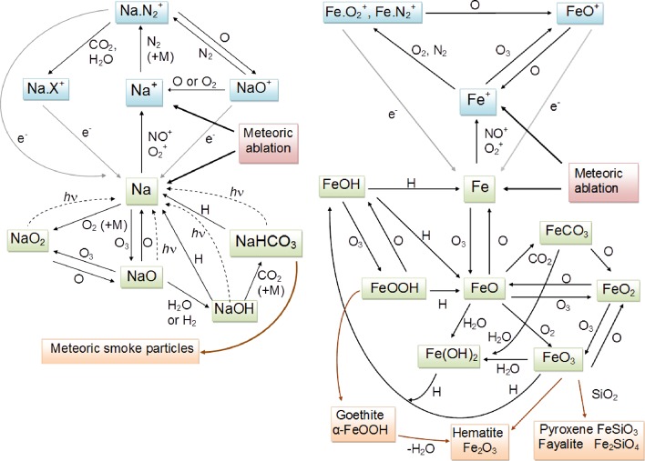
Schematic
diagrams of the chemistry of Na (left panel) and Fe (right
panel) in the mesosphere and lower thermosphere.

Map showing the locations (red stars) of ground-based
lidar observations
published since 2004. The box attached to each location indicates
the metals that have been measured and a footnote which lists the
location and a recent reference: a, South Pole; b, Syowa, Antarctica; c,
Davis, Antarctica; d, McMurdo, Antarctica; e, Rothera, Antarctica; f, Cerra Pachon, Chile; g,
São José dos Campos, Brazil; h, Kototabang, Indonesia; i, Gadanki,
India; j, Arecibo, Puerto Rico; k, Maui, HI; l,
Hefei, China; m, Wuhan, China; n, Uji, Japan; o, Albuquerque, NM; p, Beijing; q, Boulder, CO; r, Ft. Collins, CO; s, Vancouver,
Canada; t, Kühlungsborn, Germany; u, Poker Flat, AK; v, Sondrestrom, Greenland; w, Andøya,
Norway; x, Tromsø, Norway; y, Spitsbergen, Norway.

Seasonal variation of the monthly mean Fe concentration (103 cm–3) at Wuhan, China (30° N) (a,
lidar measurements; b, WACCM-Fe simulation) and at the South Pole
(c, lidar measurements; d, WACCM-Fe simulation). Adapted with permission
from ref (130). Copyright
2013 John Wiley & Sons, Inc.

Removal of metal atoms in the presence of NLC
ice particles. (a)
Simultaneous observations of the atomic Fe density and NLC backscatter
signal at the South Pole on Jan 19, 2000, made with an Fe Boltzmann
lidar operating at 372 and 374 nm, respectively. The PMC backscatter
signal is expressed as equivalent Fe atoms per cubic centimeter for
comparison with the atomic Fe resonance fluorescence signal. Adapted
with permission from ref (134). Copyright 2004 American Association for the Advancement
of Science. (b) Comparison of K profiles measured by lidar at Spitsbergen,
Norway (79° N), with a 1-D model for early May (pre-NLC seasons,
gray lines) and July (peak of the NLC season, black lines). The monthly
data are averaged over 3 years (2001–2003). Adapted with permission
from ref (138). Copyright
2007 John Wiley & Sons, Inc.

Fe Boltzmann
lidar measurements at McMurdo, Antarctica (78°
S), on May 28, 2011: (a) contour of thermospheric Fe densities from
110 to 155 km, showing fast gravity waves in the thermosphere; (b)
contour of Fe temperatures from 75 to 115 km, showing waves in the
MLT region; (c) vertical profile of temperatures for 1 h of integration
around 15 UT (universal time). The temperature errors plotted as horizontal
bars are less than 5 K below 110 km. Rayleigh lidar temperatures are
plotted below 70 km. The MSIS00 model is a standard semiempirical
atmospheric model. Reprinted with permission from ref (114). Copyright 2011 John
Wiley & Sons, Inc.

Na and Fe
density profiles measured by lidar on May 18–19,
2006, at Wuhan, China (30° N). The black curves show the point
at which the high-altitude Nas peak density reached its
maximum value. The blue dashed curves are the mean layer profiles
during that night. Note that the Fes layer had a peak density
much larger than that of the main Fe layer, while the Nas layer was slightly smaller in peak density than the main Na layer.
Reprinted with permission from ref (145). Copyright 2010 Elsevier.

Annual mean
profiles of the dynamical (blue), chemical (green),
and eddy (red) transport coefficients for atomic Na measured at the
Starfire Optical Range (35° N). Reprinted with permission from
ref (170). Copyright
2010 John Wiley & Sons, Inc.

Fe lidar
measurements between 70 and 120 km, recorded over a period
of 30 h at the ALOMAR observatory, Norway (69° N). Note the appearance
of Fe between 70 and 78 km when the mesosphere is sunlit (solar elevation
angle >−9°). Provided courtesy of J. Höffner
(Leibniz-Institute
of Atmospheric Physics (IAP), Kühlungsborn, Germany).

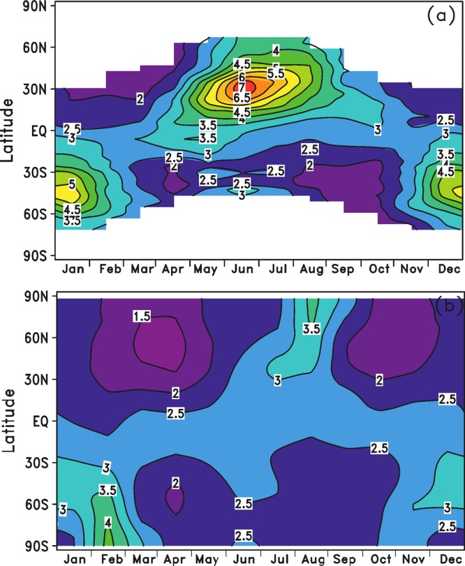
Na column abundance (109 atoms cm–2) as a function of latitude and month: (a) a Na reference atmosphere derived mostly from observations using the
Na d line at 590 nm in the dayglow; (b) WACCM-Na model results
averaged from 2004 to 2011.

K column abundance (107 atoms
cm–2) as a function of latitude and month: (a) observations
using the
K d 1 line at 769.9 nm in the dayglow; (b) WACCM-K model results, averaged from 2004
to 2011.
Mg+ column abundance (109 atoms
cm–2) as a function of latitude and month: (a) observations
using the
Mg+ line at 279 nm in the dayglow; (b) WACCM-Mg model results,
averaged from 2004 to 2011.

Nightglow spectrum (light gray line) between
500 and 700 nm recorded
on the ESI spectrometer on the Keck II telescope in Mauna Kea, HI. The spectrometer has a resolution (λ/Δ)
of 7000 and a wavelength accuracy of 0.005 Å. The red line is
a laboratory spectrum of the FeO “orange arc” emission
bands, red-shifted by 5 nm, which may
indicate different vibrational development of the excited state(s)
of FeO involved in the emission.

(a) Histogram
of the occurrence frequency of Na d line
ratio measurements. A total of 706 measurements were made between
Oct 7 and Nov 19, 2007. The solid line is a fitted three-parameter
Gaussian. (b) Correlation diagram for the electronic potential energy
surfaces connecting the reactants NaO(A) + O and NaO(X) + O with the
products Na + O2, through the NaO2 intermediate.
Quartet surfaces have been omitted for clarity; these are highly repulsive
states which do not influence the electronic nature of the products.
(c) Laboratory study of the dependence of RD on the ratio [O]/[O2]. The experimental data (solid points)
are from Slanger et al. The solid line
is a fit using the reaction scheme R38–R41.
Adapted with permission from ref (198). Copyright 2012 Elsevier.

Rocket-borne study of
the Na layer and charged MSPs. (a) Comparison
of the atomic O profile measured by the NEMI instrument on the HotPay
2 rocket payload, with the Na density measured by the ground-based
ALOMAR Na lidar 5 min before the rocket launch. The payload passed
within 2.58 km of the lidar at an altitude of 90 km. (b) Comparison
of the profiles of positive ions and electrons measured by an ion
probe and Faraday rotation technique on HotPay 2, compared with the
predictions of the plasma model (including a profile of negative ions).
The removal of electrons between 80 and 90 km is due to the charging
of MSPs. (c) Vertical profile of negatively charged aerosols measured
by a dust detector on HotPay 2, compared with the prediction from
the dusty plasma model. The difference between the measured positive
ions and electrons in (b) is also shown. Adapted with permission from
ref (125). Copyright
2014 Elsevier.

MSP work function. (a) Photoelectron currents
measured during the
flight of rocket payload ECOMA08. Black, green, and red symbols indicate
the currents produced by the three different flashlamps (see the legend),
where FX1162, FX1161, and FX1160 have cutoff wavelengths at 110, 190,
and 225 nm, respectively. The dotted horizontal line marks the 2σ
noise level of the unsmoothed measurements. (b) Optimized geometries
of possible embryonic meteoric smoke particles: (FeOH)4, (MgOH)4, (FeSiO3)3, and (Mg2SiO4)4. The vertical ionization potentials
are shown alongside each cluster. Note that these are 2 eV larger
when the cluster contains a silicon atom. Adapted with permission
from ref (215). Copyright
2012 Copernicus Publications on behalf of the European Geosciences
Union.

Comparison
of measured MSP extinction (labeled SOFIE/AIM) with
values calculated using MSP number concentrations from the UMSLIMCAT
model and Rayleigh theory for an assumed olivine (MgFeSiO4) composition and for the same pyroxene (Mg0.4Fe0.6SiO4) species used to fit the SOFIE data by Hervig et
al. Also shown are the predicted MSP
extinction profiles from the WACCM and
CHEM2D models. Reprinted with permission
from ref (279). Copyright
2012 Copernicus Publications on behalf of the European Geosciences
Union.

(a) Schematic diagram
of the pulsed laser photolysis/laser-induced
fluorescence detection apparatus used to study the reactions of Mg+ ions. The metal precursor (magnesium acetyl acetonate) is
placed in a tantalum boat in the side arm of the reactor. PMT = photomultiplier
tube, MC = monochromator, PD = photodiode, and BE = beam expander.
(b) Time-resolved profile of the LIF signal obtained by pumping the
Mg+(32P1)–Mg+(31S0) transition at 279.6 nm and monitoring emission
at the same wavelength, following the pulsed photolysis at 193.3 nm
of magnesium acetyl acetonate. The solid line is a fit to the form A exp(−k′t).

Schematic diagram of a fast flow tube apparatus
used to study the
reactions of neutral Ca (probed by LIF at 422.7 nm) and CaO (probed
by LIF at 385.9 nm). P = photomultiplier tube. I1, I2, and I3 are
reagent inlets.

Photoionization cross-section of Na atoms adsorbed on
ice (black
points and line), compared with gas-phase
Na atoms (red line). The blue line is
the solar photon flux (right-hand ordinate).

(a) Experimental
system used for the photochemical generation,
detection, capture and optical extinction measurements of MSP mimics.
(b) Transmission electron microscopy images and an electron diffraction
image taken from the indicated area within a smoke aggregate formed
following the irradiation of a mixture of Fe(CO)5, O3/O2, and tetraethyl orthosilicate. Adapted with
permission from ref (201). Copyright 2006 Elsevier.

Ablation/sputtering
profiles of individual elements from a 5 μg
meteoroid entering the atmosphere at 20 km s–1 and
at 37° to the zenith. The particle temperature is shown with
the solid black line, referenced to the top abscissa. Adapted with
permission from ref (96). Copyright 2008 Copernicus Publications on behalf of the European
Geosciences Union.

An observed meteor with
the following best fit parameters: initial
velocity 36 km s–1; entry angle 1° (to zenith);
mass 10–8 kg; density 3500 kg m–3. (a) Meteor range-time intensity, measured with the 430 MHz Arecibo
radar. (b) Modeled (line) and observed (tilted squares) meteor altitude–velocity
profile. (c) Modeled (black) and observed (red) meteor signal-to-noise
ratio. (d) Modeled meteor radar cross-section. (e) Ablation profiles
of the main elements (bottom axis) and total amount of electrons produced
(upper axis), predicted by CABMOD. The
horizontal line across the plots shows that the observed enhancement
in SNR is due to the rapid ablation of the alkali metals Na and K.
Reprinted with permission from ref (261). Copyright 2009 John Wiley & Sons, Inc.

(a) Meteoric ablation flux of Fe (cm–2 s–1) as a function of latitude and season. (b)
Global
annual mean Fe injection rate (cm–3 s–1) as a function of height. Adapted with permission from ref (130). Copyright 2013 John
Wiley & Sons, Inc.

Three days of WACCM-Fe model output sampled every 30 min
for Urbana
from July 1, 2005: (a) temperature (K); (b) Fe mixing ratio (pptv);
(c) perturbation in temperature (difference from the 3-day average);
(d) perturbation in Fe mixing ratio. The time in the plot is universal
time (UT). Local time = UT – 6 h. Adapted with permission from
ref (130). Copyright
2013 John Wiley & Sons, Inc.

WACCM total column Na (cm–2) at 0000 UT on Jan
22 and Feb 6, 2009. A major sudden stratospheric warming event occurred
on Jan 24. Reprinted with permission from ref (188). Copyright 2013 John
Wiley & Sons, Inc.

Zonal average plots
for January (top) and July (bottom) of the
MSP concentration, mass density, and effective radius for the control
simulation. The data are an average of the last 7 years of a 10 year
simulation using WACCM coupled to the CARMA aerosol microphysics model.
The effective radius is calculated as the ratio of the third and second
moments of the dust size distribution. Reprinted with permission from
ref (278). Copyright
2008 John Wiley & Sons, Inc.

Map
of the annual mean Fe deposition rate (μmol of Fe m–2 year–1) of mesospheric Fe from
MSPs. Reprinted with permission from ref (232). Copyright 2013 John Wiley & Sons, Inc.
References
-
- Plane J. M. C. Int. Rev. Phys. Chem. 1991, 10, 55.
-
- Plane J. M. C. Chem. Rev. 2003, 103, 4963. - PubMed
-
- Plane J. M. C.; Helmer M. In Research in Chemical Kinetics; Compton R. G., Hancock G., Eds.; Elsevier Science: Amsterdam, 1994.
-
- Plane J. M. C. In Meteors in the Earth’s Atmosphere; Murad E., Williams I. P., Eds.; Cambridge University Press: Cambridge, U.K., 2002.
-
- McNeil W. J.; Murad E.; Plane J. M. C. In Meteors in the Earth’s Atmosphere; Murad E., Williams I. P., Eds.; Cambridge University Press: Cambridge, U.K., 2002.
Grants and funding
LinkOut - more resources
Full Text Sources
Other Literature Sources