. 2015 Mar;71(Pt 3):646-66.
doi: 10.1107/S1399004714028132. Epub 2015 Feb 26.

FEM: feature-enhanced map

Affiliations

FEM: feature-enhanced map

Pavel V Afonine et al. Acta Crystallogr D Biol Crystallogr. 2015 Mar.

Abstract

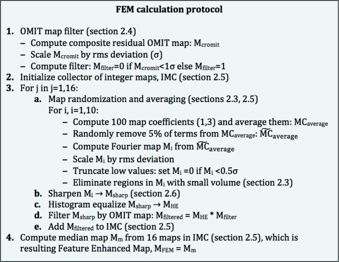
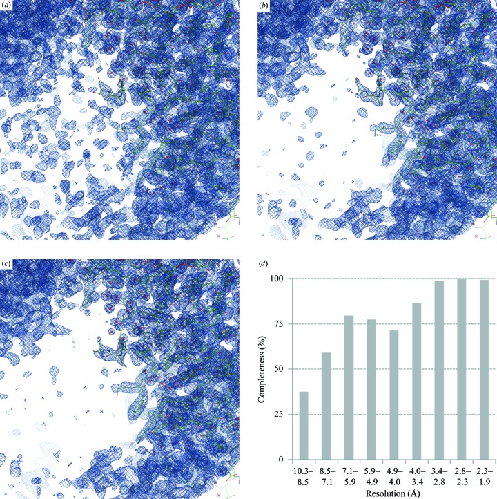
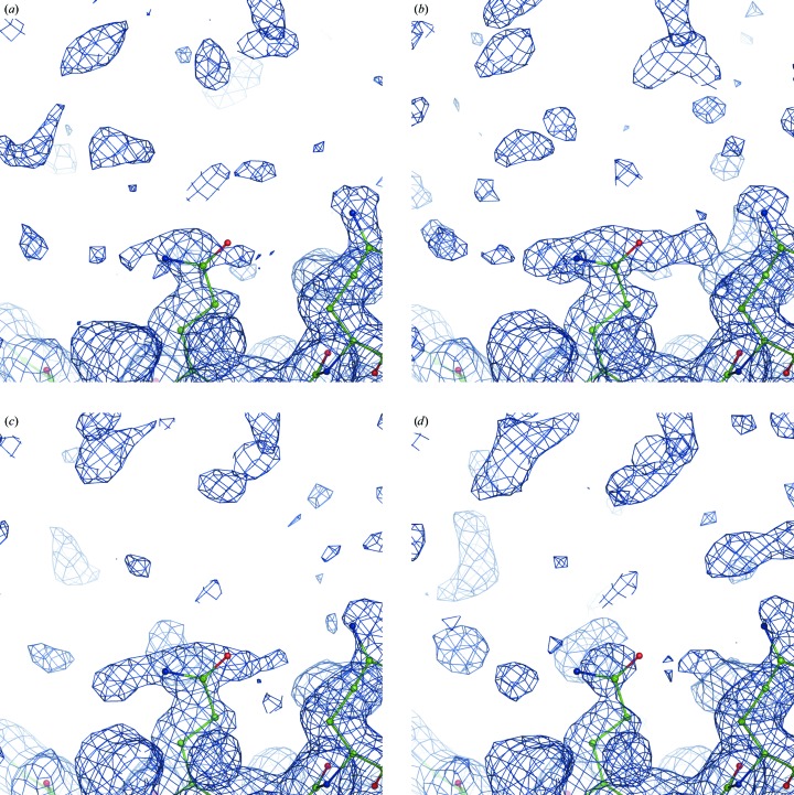
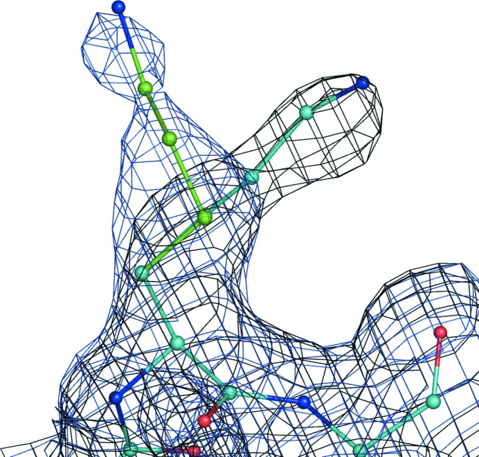
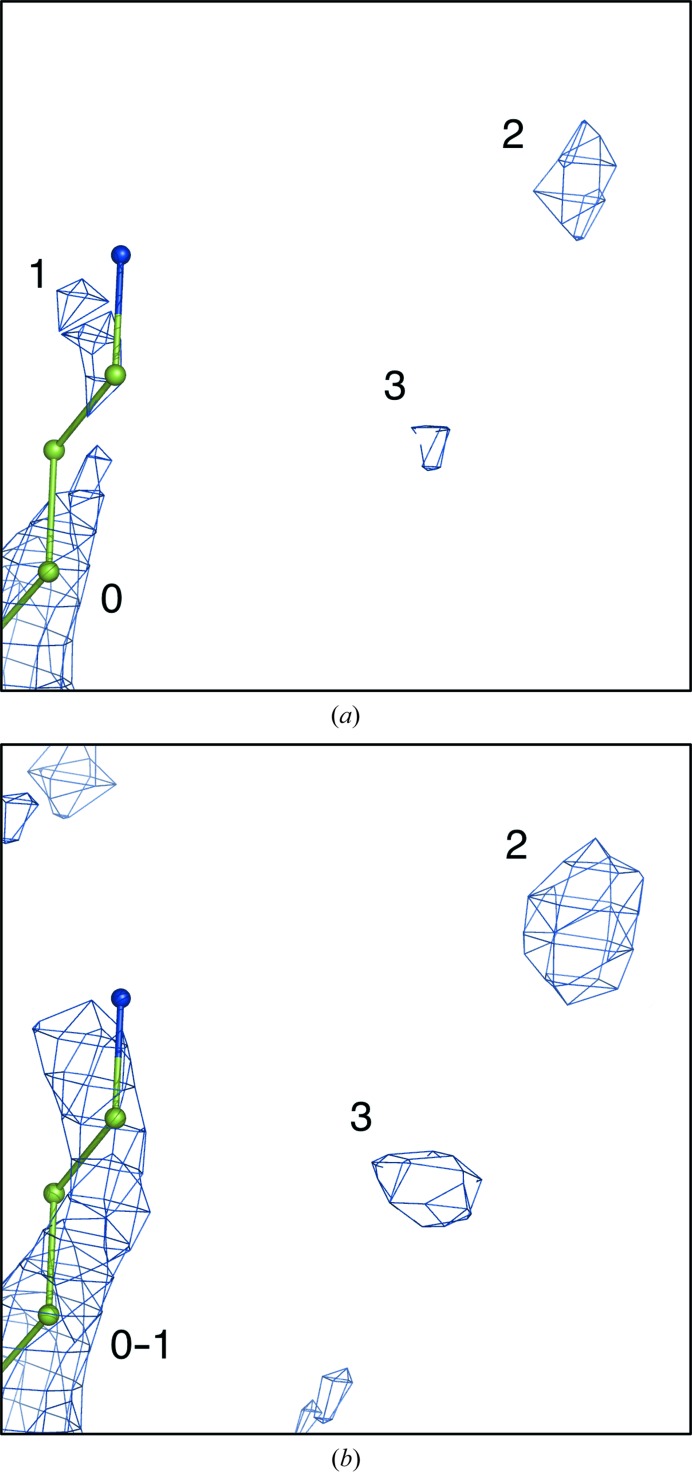
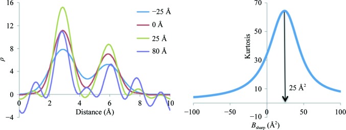
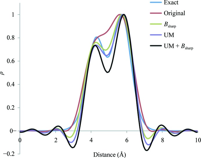
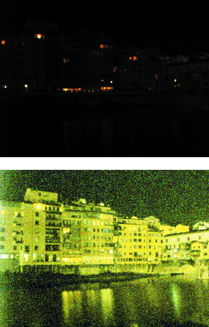
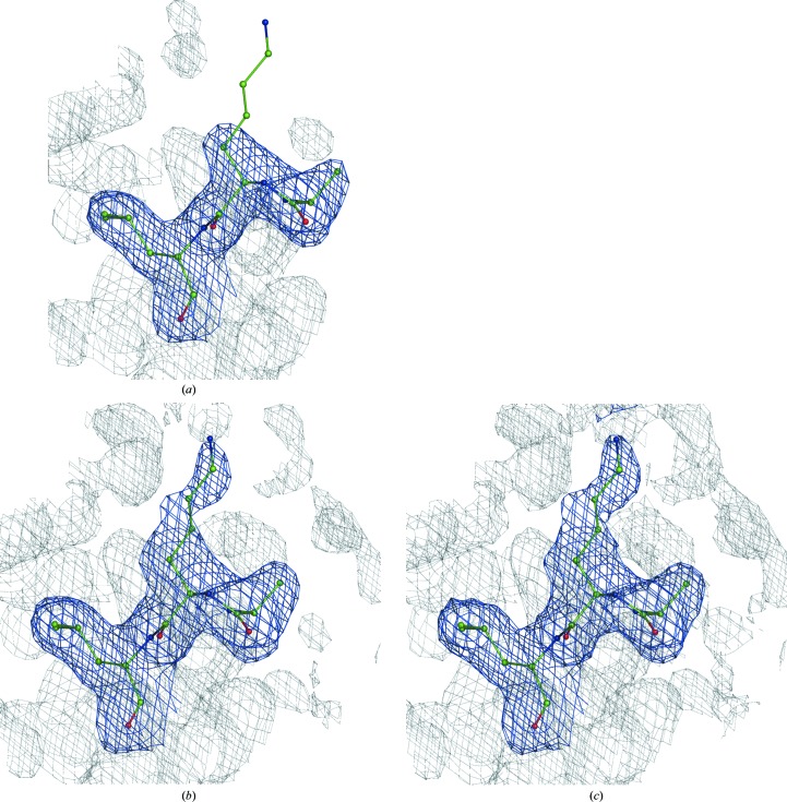
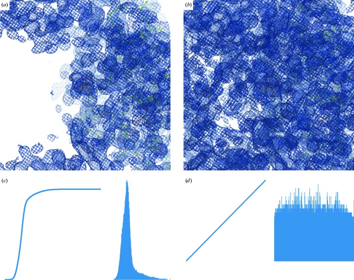
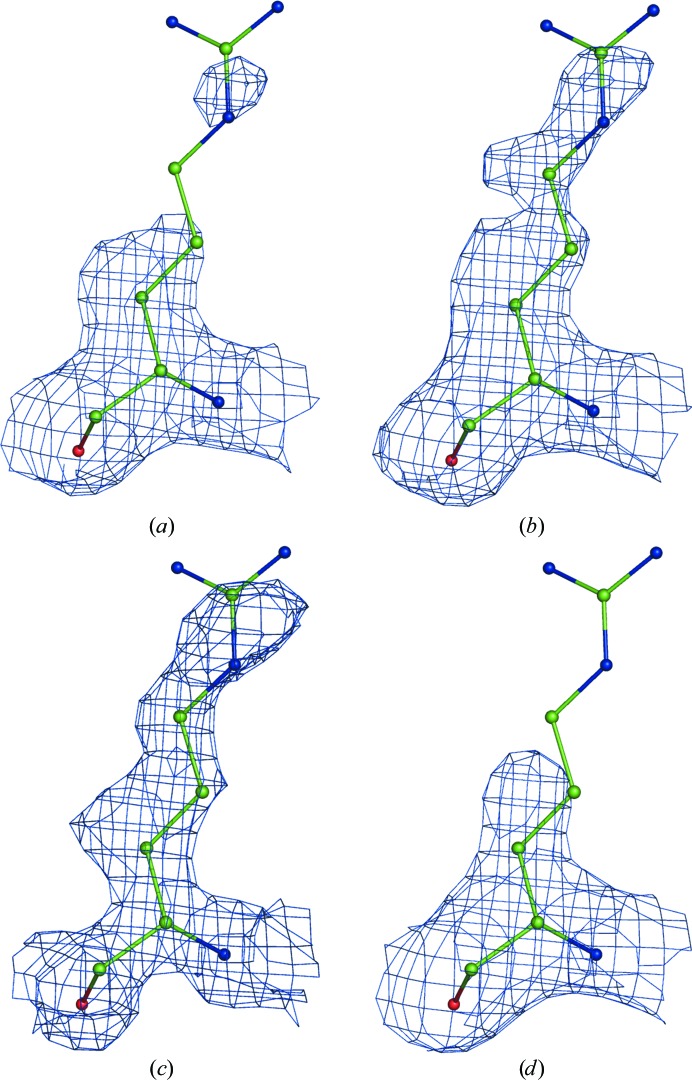
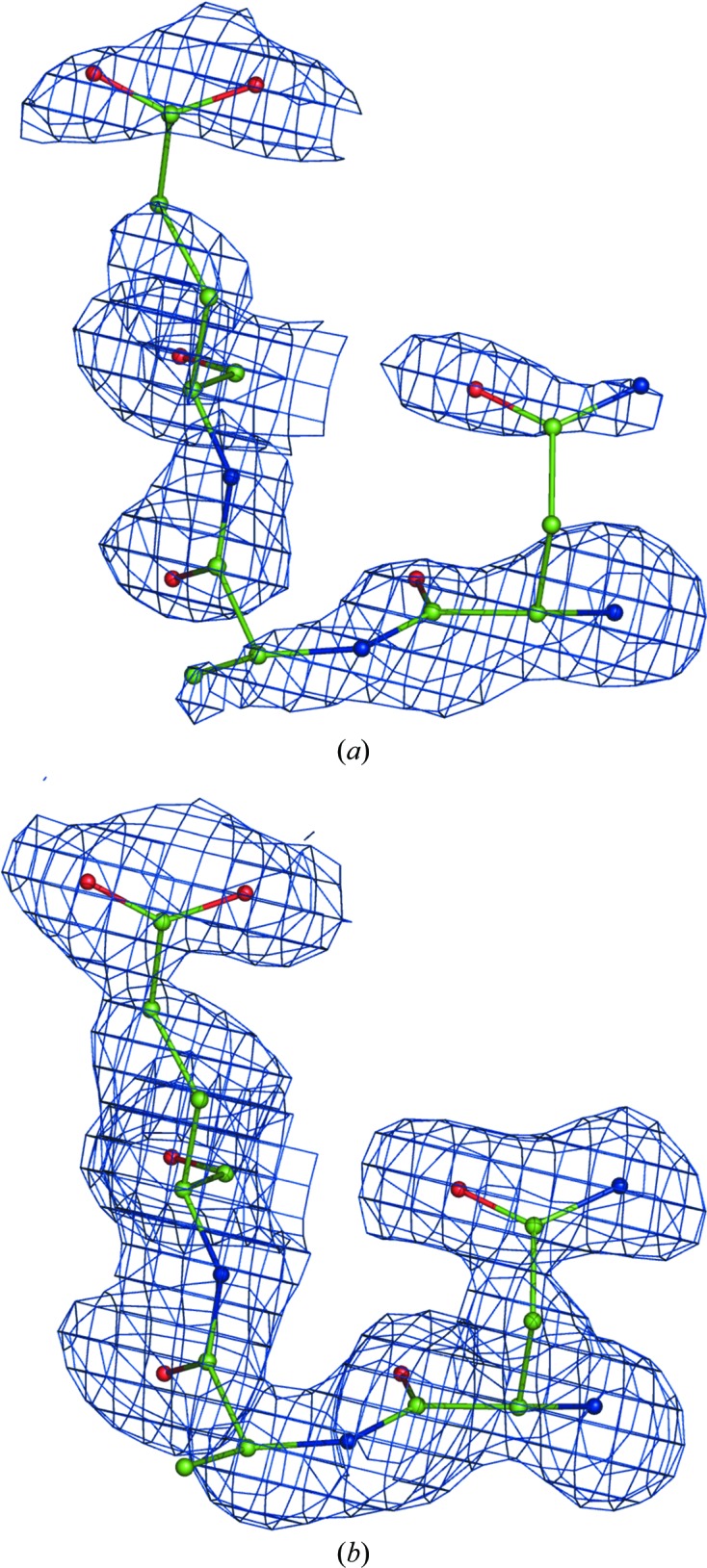
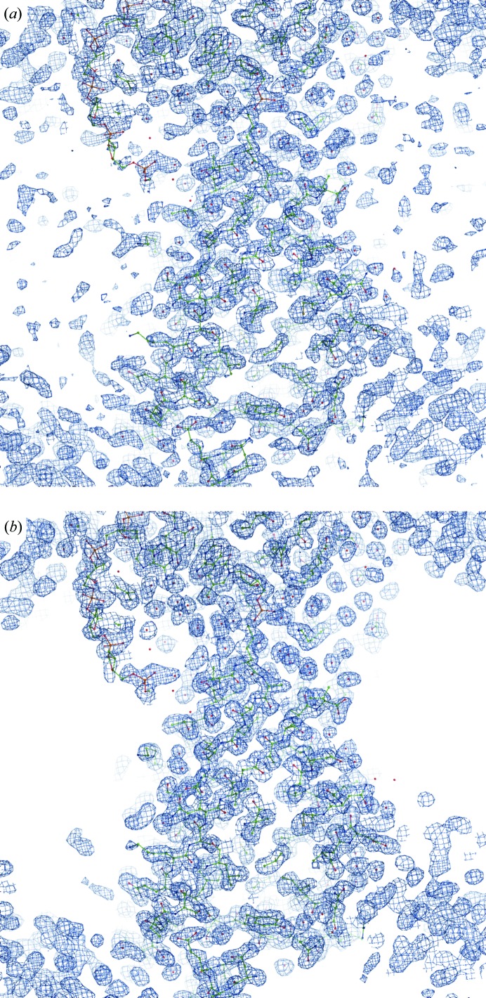
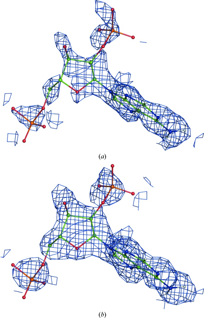
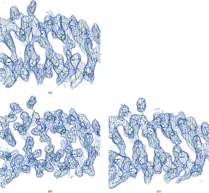
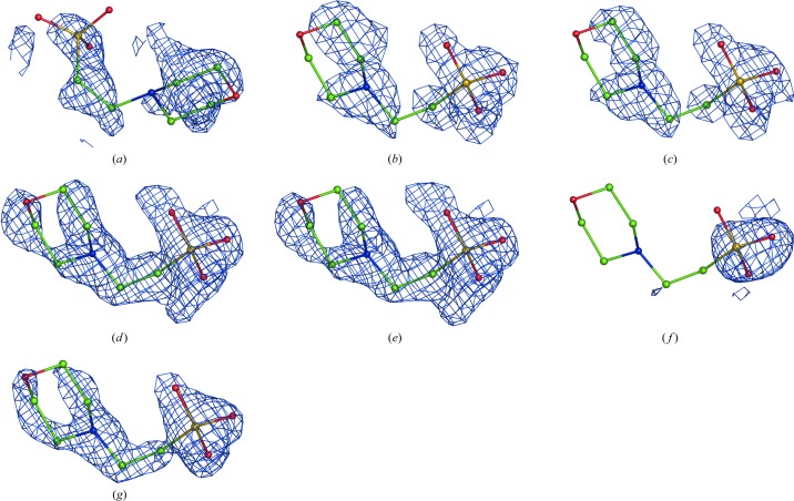
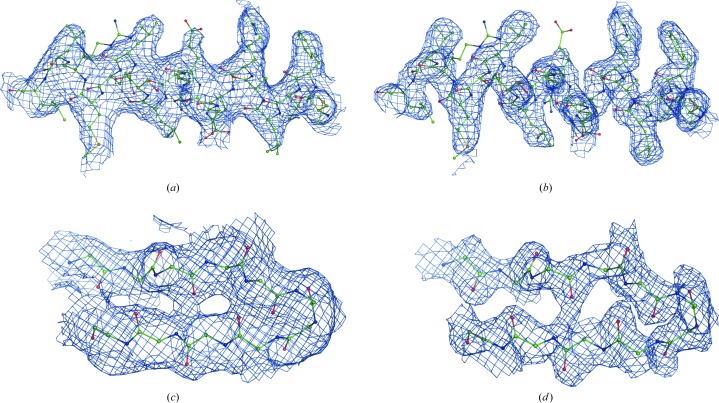
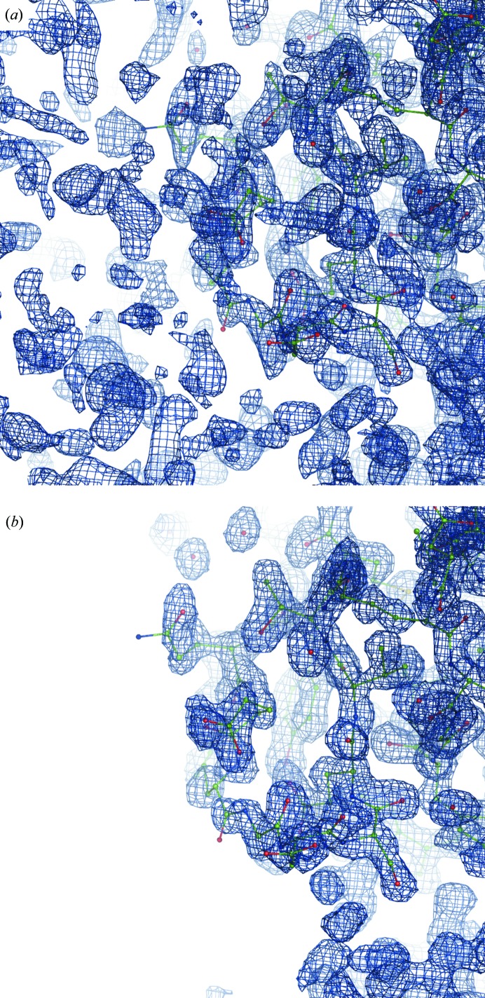
A method is presented that modifies a 2mFobs - DFmodel σA-weighted map such that the resulting map can strengthen a weak signal, if present, and can reduce model bias and noise. The method consists of first randomizing the starting map and filling in missing reflections using multiple methods. This is followed by restricting the map to regions with convincing density and the application of sharpening. The final map is then created by combining a series of histogram-equalized intermediate maps. In the test cases shown, the maps produced in this way are found to have increased interpretability and decreased model bias compared with the starting 2mFobs - DFmodel σA-weighted map.

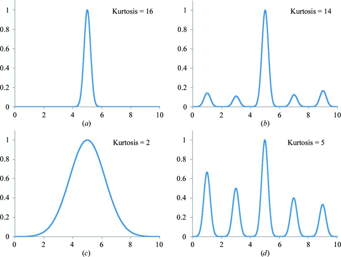
Keywords: FEM; Fourier map; OMIT; PHENIX; cctbx; density modification; feature-enhanced map; map improvement; map kurtosis; map sharpening; model bias.


Figures

Figure 1
Figure 1
FEM protocol. The individual steps are explained in the corresponding sections of the manuscript.
Figure 2
Figure 2
The effect of missing data and its restoration for PDB entry 1nh2: maps calculated using (1) with (a) F fill = 0 (1.0σ), (b) F fill derived from a RESOLVE density-modified map (1.1σ) and (c) F fill derived from the model as described in §2.2 (1.0σ). (d) Resolution-bin completeness of the diffraction data for PDB entry 1nh2. Note the very poor completeness at low resolution and the rather good overall completeness, which is 95% in the range (1.9, ∞). Log-scale binning is used as described in Afonine, Grosse-Kunstleve et al. (2013 ▶), which efficiently highlights poor low-resolution completeness. See §2.9 regarding the choice of map-contouring levels.
Figure 3
Figure 3
Fourier maps calculated with (1): (a) w = 1 (0.5σ), (b, c) w computed using (3) (0.45σ), (d) the same as (c) but with 5% of the terms omitted. Note that the signal (the density around the atoms) is similar while the noise (the density further away from the atoms) is reshuffled in all four cases. See §2.9 regarding the choice of contouring threshold levels.
Figure 4
Figure 4
The correct residue Lys107 (chain L) of PDB entry 1f8t (the rotamer on the left) is shown as a blue map calculated using (1) with w = 1. The same residue side chain switched to an incorrect rotamer (right) is shown as a black map calculated using (1) with weights from (3) with δ = 1.5. Both maps are contoured at 1σ. Clearly, the black map is model-biased as it follows the wrong side-chain orientation and otherwise coincides with the correct (blue) map.
Figure 5
Figure 5
Schematic illustration of the elimination of noise peaks. (a) Map contoured at a threshold level t 1: blobs 1, 2 and 3 are selected for elimination, while blob 0 is retained. (b) Map contoured at a threshold level t 2 = t 1 − δ. We note that blob 1 merges with blob 0 and is therefore retained, while the larger blobs 2 and 3 are removed.
Figure 6
Figure 6
Composite residual OMIT map-calculation workflow. See §2.4 for details.
Figure 7
Figure 7
Testing the performance of the OMIT map-calculation procedure. Model 1 consists of two residues, 1 and 2, placed in a P1 box and is used to calculate the (F A, ϕA) synthesis (a). Model 2 consists of one residue, 1 (otherwise identical to model 1), and is used to calculate the (F B, ϕB) synthesis (b). Amplitudes F B and phases ϕA are used to compute synthesis (c). All syntheses are contoured at 3σ. The positive map around residue 2 in (c) is purely model bias.
Figure 8
Figure 8
Relationships between map kurtosis and model B factor and data resolution. (a) Fourier map values of resolution 1.5 Å along the Mg—O bond shown for three selected B-factor values: 10, 30 and 50 Å2. (b) Map kurtosis shown as a function of the B factor. (c) Fourier map values of resolutions 1, 2 and 3 Å along the Mg—O bond. (d) Map kurtosis shown as a function of resolution.
Figure 9
Figure 9
Illustrations of kurtosis for four different functions.
Figure 10
Figure 10
Left, distribution of Fourier map values of resolution 1.5 Å along the Mg—O bond corresponding to different sharpening B factors (B sharp). Right, map kurtosis as function of B sharp.
Figure 11
Figure 11
Effect of map sharpening using unsharp masking and exponential (B-factor) sharpening methods. See §2.6.2 for details. For easier comparison all maps are scaled to have their maximum value equal to 1.
Figure 12
Figure 12
Illustration of histogram equalization. An underexposed night photograph (top) and its histogram-equalized version (bottom) (the pictures were taken by the first author). Although the HE picture is unrealistic (i.e. it gives a false impression that it is daytime) it does shows significantly more detail than the original image.
Figure 13
Figure 13
Illustration of histogram equalization. Weak side-chain density for residue Lys83 in chain A of PDB entry 1ssw. The synthesis in (1) was contoured at 1σ (a) and 0.4σ (b). (c) HE map contoured at a level equivalent to 1σ. Blue, only density within a 1.5 Å radius around atoms is shown; grey, the same as the blue map but shown within a 5 Å radius around atoms. The blue map is shown on top of the grey map.
Figure 14
Figure 14
Illustration of histogram equalization for PDB entry 2bwl. First row, original map from (1) contoured at 1.3σ (left) and the HE map (right) at the same contour level. Second row, histogram and cumulative histogram of the synthesis values: left, original map; right, HE map.
Figure 15
Figure 15
Fourier map distribution along the Mg—O—H line (blue) and its histogram-equalized version (red). Left, original map; right, map truncated with ρtrunc = 0 if ρ < 0.05. Note the enhancement of noise peaks as a result of applying HE (left, red line).
Figure 16
Figure 16
Schematic illustration of choosing equivalent map-contouring thresholds. The red and blue curves are cumulative distribution functions (CDFs) corresponding to the two r.m.s. deviation-scaled maps in question. Given the contouring threshold for map 1 (σ1), first one needs to find the corresponding value of the CDF. Next, one looks up the contouring threshold of map 2 (σ2) that corresponds to the same value of the CDF as for map 1. The contouring thresholds σ1 and σ2 encompass equivalent fractions of both maps.
Figure 17
Figure 17
Maps for PDB entry 1f8t residue Arg74 (chain L). (a) Map from (1) at 1.0σ. (b) Composite residual OMIT map from (2) at 1.5σ calculated as described in §2.4. (c) FEM contoured at 1.1σ. (d) RESOLVE density-modified map at 0.8σ.
Figure 18
Figure 18
Maps for PDB entry 1nh2. (a) Map from (1) at 1.0σ. (b) FEM contoured at the equivalent to 1.0σ. Residues 3–5 of chain B are shown.
Figure 19
Figure 19
View of macromolecule and bulk-solvent areas for PDB entry 1nh2. The map from (1) (a) and the FEM (b) contoured at 1.0σ. The macromolecule and the bulk-solvent interface are shown.
Figure 20
Figure 20
Neutron structure of aldose reductase (PDB entry 2r24). A fragment of the NAP ligand in the nuclear map is shown. (a) is the map from (1) and (b) is the FEM; both are contoured at 1σ.
Figure 21
Figure 21
(a) The original map from (1), (b) the FEM and (c) a RESOLVE density-modified map for PDB entry 2g38, where the data are known to be affected by severe anisotropy. Note the reduction in the effect of map anisotropy along the vertical direction in both the FEM and RESOLVE maps.
Figure 22
Figure 22
An example of a misfitted ligand in PDB entry 1se6. (a) The incorrect fit shown in the map from (1). The FEM is shown calculated with (b) and without (c) the incorrectly fitted ligand included in the calculations. The composite residual OMIT map is shown with (d) and without (e) the incorrectly fitted ligand included in the calculations. (f) RESOLVE density-modified map. (g) Ligand-omit map from (1) after correcting the ligand fit followed by a round of refinement. All maps are shown at 1σ or equivalent.
Figure 23
Figure 23
Feature-enhanced maps (FEMs) without sharpening (a, c) and with sharpening (b, d). (a, b) PDB model 2vui, residues 123–140 of chain B. (c, d) PDB model 2ppi, residues 32–43 of chain A. All maps are contoured at 1σ.
Figure 24
Figure 24
(a) Map from (1) and (b) FEM for PDB entry 3i9q, both contoured at 1σ.
Figure 25
Figure 25
The first 100 models from an ensemble of 1000 MD-generated models, illustrating the diversity of starting points for real-space refinement (see §3.7 for details). Backbone atoms are shown in black.
Figure 26
Figure 26
Distribution of r.m.s. deviations between real-space refined models and the best available model: refinements against FEM (blue) and against the map from (1) (red). Clearly, the majority of structures refined closer to the true structure when the FEM was used as a target map.

References

    1. Abramowitz, M. & Stegun, I. A. (1972). Handbook of Mathematical Functions with Formulas, Graphs, and Mathematical Tables, p. 928. New York: Dover.
    1. Adams, P. D. et al. (2010). Acta Cryst. D66, 213–221. - PubMed
    1. Afonine, P. V., Grosse-Kunstleve, R. W. & Adams, P. D. (2005). Acta Cryst D61, 850–855. - PMC - PubMed
    1. Afonine, P. V., Grosse-Kunstleve, R. W., Adams, P. D. & Urzhumtsev, A. (2013). Acta Cryst. D69, 625–634. - PMC - PubMed
    1. Afonine, P. V., Grosse-Kunstleve, R. W., Echols, N., Headd, J. J., Moriarty, N. W., Mustyakimov, M., Terwilliger, T. C., Urzhumtsev, A., Zwart, P. H. & Adams, P. D. (2012). Acta Cryst. D68, 352–367. - PMC - PubMed

Publication types

MeSH terms