Speed of conformational change: comparing explicit and implicit solvent molecular dynamics simulations

Abstract

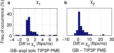
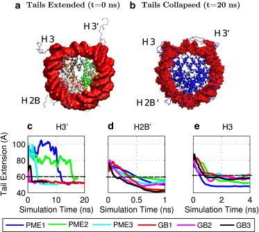
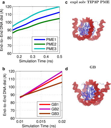
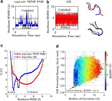
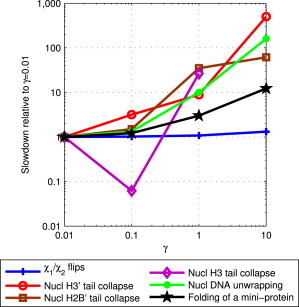
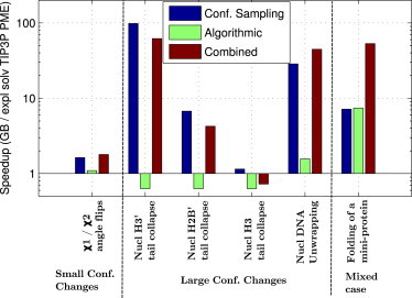
Adequate sampling of conformation space remains challenging in atomistic simulations, especially if the solvent is treated explicitly. Implicit-solvent simulations can speed up conformational sampling significantly. We compare the speed of conformational sampling between two commonly used methods of each class: the explicit-solvent particle mesh Ewald (PME) with TIP3P water model and a popular generalized Born (GB) implicit-solvent model, as implemented in the AMBER package. We systematically investigate small (dihedral angle flips in a protein), large (nucleosome tail collapse and DNA unwrapping), and mixed (folding of a miniprotein) conformational changes, with nominal simulation times ranging from nanoseconds to microseconds depending on system size. The speedups in conformational sampling for GB relative to PME simulations, are highly system- and problem-dependent. Where the simulation temperatures for PME and GB are the same, the corresponding speedups are approximately onefold (small conformational changes), between ∼1- and ∼100-fold (large changes), and approximately sevenfold (mixed case). The effects of temperature on speedup and free-energy landscapes, which may differ substantially between the solvent models, are discussed in detail for the case of miniprotein folding. In addition to speeding up conformational sampling, due to algorithmic differences, the implicit solvent model can be computationally faster for small systems or slower for large systems, depending on the number of solute and solvent atoms. For the conformational changes considered here, the combined speedups are approximately twofold, ∼1- to 60-fold, and ∼50-fold, respectively, in the low solvent viscosity regime afforded by the implicit solvent. For all the systems studied, 1) conformational sampling speedup increases as Langevin collision frequency (effective viscosity) decreases; and 2) conformational sampling speedup is mainly due to reduction in solvent viscosity rather than possible differences in free-energy landscapes between the solvent models.

Figure 1

Difference in (a) χ₁ and (b) χ₂ dihedral angle flips (GB − explicit-solvent (TIP3P) PME) from 770 ns simulations of 1GYM protein. Flips are measured as changes in dihedral angles across distinct ranges of dihedral angles, as described in the text. To see this figure in color, go online.

Figure 2

Three sets of independent MD simulations of the nucleosome tail collapse. (a) PDB structure with three histone tails (H3, H3′, and H2B′) extended. (b) Structure with the positively charged histone tails collapsed onto the negatively charged DNA. DNA surface is shown in red and the histone backbone structure is shown in blue. Tail extension is measured as the distance from the N-terminus tail to the center of geometry of the DNA. (c–e) Results show moving average values, averaged over 0.5 ns, from three explicit-solvent (TIP3P) PME and GB simulations. Connecting lines are shown to guide the eye. Images were rendered using VMD (100). To see this figure in color, go online.

Figure 3

Nucleosome DNA unwrapping at high pH. (a and b) DNA end-to-end distance for three explicit-solvent (TIP3P) PME (a) and GB (b) simulations. Moving average values, averaged over 0.5 ns, are shown, with connecting lines to guide the eye. (c) Ends of the DNA unwrapped from the histone core after 0.8 ns of an explicit-solvent (TIP3P) PME simulation. (d) Ends of the DNA unwrapped from the histone core after 0.03 ns of a GB simulation. DNA surface is shown in red and histone backbone structure in blue. Images were rendered using VMD (100). To see this figure in color, go online.

Figure 4

CLN025 miniprotein folding at its experimental melting temperature of 340 K. (a and b) RMSD of backbone heavy atoms relative to the starting structure for the explicit-solvent (TIP3P) PME simulation (a) and the GB simulation (b). The horizontal lines represent RMSD = 1.5 and 4.5 Å. Folded states are states with RMSD < 1.5 Å and unfolded states are states with RMSD > 4.5 Å. The trajectory is sampled every 100 ps for calculation of the RMSD values shown here. (c) Free-energy landscape for the explicit-solvent TIP3P PME and the GB simulations. (d) Potential energy, including solvation free energy, from the GB simulation, as a function of the distance (RMSD) from the experimental native structure. The lowest-energy structure approximates the correct folded state, as indicated by the low RMSD values. (Inset) Images of protein backbone conformations from representative snapshots for folded and unfolded states from the explicit-solvent (TIP3P) PME (blue) and GB (red) simulations. The starting structure (green) is shown for comparison. Images rendered using VMD (100). To see this figure in color, go online.

Figure 5

Effect of Langevin dynamics collision frequency, γ, on conformational sampling speed of GB simulations. Slowdown is computed relative to the average speed of conformational change at the baseline value of γ = 0.01 ps⁻¹. The H3 histone tail did not collapse for γ = 10 ps⁻¹, even after 22 ns of simulation (over 20 days of wall clock time), and therefore, this data point is not shown. Connecting lines shown to guide the eye. To see this figure in color, go online.

Figure 6

Average speedup for GB relative to explicit-solvent (TIP3P) PME simulations. The combined speedup includes the average speedup due to differences in the rate of conformational sampling, as well as due to algorithmic differences between the two methods. The Langevin dynamics collision frequency of γ = 0.01 ps⁻¹ was used for these simulations. To see this figure in color, go online.

References

1. Dodson G.G., Lane D.P., Verma C.S. Molecular simulations of protein dynamics: new windows on mechanisms in biology. EMBO Rep. 2008;9:144–150. - PMC - PubMed
1. Karplus M., Kuriyan J. Molecular dynamics and protein function. Proc. Natl. Acad. Sci. USA. 2005;102:6679–6685. - PMC - PubMed
1. Dror R.O., Dirks R.M., Shaw D.E. Biomolecular simulation: a computational microscope for molecular biology. Annu. Rev. Biophys. 2012;41:429–452. - PubMed
1. Wang W., Donini O., Kollman P.A. Biomolecular simulations: recent developments in force fields, simulations of enzyme catalysis, protein-ligand, protein-protein, and protein-nucleic acid noncovalent interactions. Annu. Rev. Biophys. Biomol. Struct. 2001;30:211–243. - PubMed
1. Schlick T., Collepardo-Guevara R., Xiao X. Biomolecular modeling and simulation: a field coming of age. Q. Rev. Biophys. 2011;44:191–228. - PMC - PubMed
Publication types