Estimating cellular parameters through optimization procedures: elementary principles and applications

Abstract

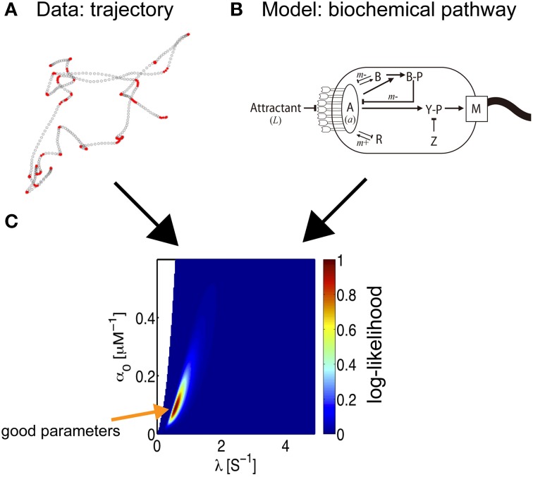
Construction of quantitative models is a primary goal of quantitative biology, which aims to understand cellular and organismal phenomena in a quantitative manner. In this article, we introduce optimization procedures to search for parameters in a quantitative model that can reproduce experimental data. The aim of optimization is to minimize the sum of squared errors (SSE) in a prediction or to maximize likelihood. A (local) maximum of likelihood or (local) minimum of the SSE can efficiently be identified using gradient approaches. Addition of a stochastic process enables us to identify the global maximum/minimum without becoming trapped in local maxima/minima. Sampling approaches take advantage of increasing computational power to test numerous sets of parameters in order to determine the optimum set. By combining Bayesian inference with gradient or sampling approaches, we can estimate both the optimum parameters and the form of the likelihood function related to the parameters. Finally, we introduce four examples of research that utilize parameter optimization to obtain biological insights from quantified data: transcriptional regulation, bacterial chemotaxis, morphogenesis, and cell cycle regulation. With practical knowledge of parameter optimization, cell and developmental biologists can develop realistic models that reproduce their observations and thus, obtain mechanistic insights into phenomena of interest.

Keywords: likelihood; model selection; parameter optimization; probability density function; quantitative modeling.

Figure 1

Correlation analyses between parameters. (A) A linear correlation and linear regression. X and Y are two parameters of a dataset. Plotting the values of Y against X shows a correlation between the parameters, and the extent of that correlation can be calculated by regression analysis. (B) The relationship between the mean square displacement (MSD) and the time lag for various modes of motion (see text for details). (C) The same plot as shown in (B), except using logarithmic values. The three lines correspond to the different modes of motion in (B). For Brownian motion, the slope of the log–log plot is one. For directional motion and sub-diffusion, the log–log plots yield a linear relationship with a slope greater than one and less than one, respectively.

Figure 2

Likelihood: the distribution is important. (A) An example of the mean of predicted values and observed data points. (B) If the distribution of the predicted values of the model is broad, the likelihood of the model is high because the probability of observing the data is high. (C) In contrast, if the distribution of the predicted value is narrow, the likelihood will be low. (D) An example of AIC calculation. Black dots represent an imaginary set of observed data. For x = 1, 2, 3, …, 20, the y value was calculated according to y = 0.025 × (x - 3) (x-10) (x − 17) + 10, and a Gaussian noise correction with a variance of four was added to each y value. Next, we calculated the best-fit linear, cubic, and fifth-order polynomial functions for the 20 data points. l_max = −(n/2) × ln(2πσ²) – (1/2σ²) × Σ_i=1ⁿ [y_i - y_model(x_i)]², where n is the number of data points (n = 20), σ² is the variance of the model, and y_i and y_model(x_i) are observed and model values, respectively, at x = x_i. The sum of squared residuals is Σ_i=1ⁿ[y_i - y_model(x_i)]². AIC is calculated as AIC = 2k − 2l_max, where k is the number of free parameters in the model and is 3, 5, and 7 for linear, cubic, and fifth-order functions, respectively. Note that the variance of each model is also a free parameter to be optimized.

Figure 3

Various optimization strategies. (A–C) Gradient approaches. (A) When the partial differential equations for likelihood can be solved as functions of parameters, the solutions yield local maxima or minima (red and gray arrows). The red arrow indicates maximum likelihood. (B) We can reach local maxima (red arrows) by iteratively following the gradient from a starting point. (C) If, in following the gradient, we add stochasticity, we may avoid being trapped in a local maximum and reach the global maximum (red arrow). (D–F) Sampling approaches. The red arrow indicates the sampling point with the highest likelihood. (D) Grid sampling, in which sampling occurs at regular intervals. (E) Simple random sampling, where parameters are chosen at random. (F) Importance sampling was added to (E). In the second round of sampling, more realizations were set near the realization with high likelihood from the initial round (gray crosses and circles).

Figure 4

Bayesian inference of parameter distribution. (A) In the sampling approach, the likelihood of observing experimental data for a realization is calculated (a, b). Then, the non-normalized posterior PDF is calculated by interpolating the likelihood values in the parameter space between the realizations (c). (B) In the gradient approach, a realization (e.g., θ₀) is randomly shifted to a neighboring realization (θ₁ or θ₁'). If the product of the likelihood and the prior probability of the new realization is greater than that of the original, the old realization will be replaced by the new realization and sampled. If the product for the new realization is smaller, the realization will be replaced by the new set, and the probability of this new set will be given as the ratio of the products of the new and the old realizations (otherwise, the original realization will not be replaced), and the realization will be sampled (a). After repeating the procedure multiple times (b), the distribution of the sampled realizations is considered proportional to the posterior PDF (c).

Figure 5

Parameter estimation of bacterial behavior. The inference of biochemical parameters in the bacterial chemotaxis pathway from trajectories (Masson et al., 2012). (A) Bacteria swimming in a microfluidic device in the presence of a stable, linear chemical gradient (here, Me-Asp) are tracked. According to the current linear speed and angular velocity, a state is associated with the bacterial motion, run (empty circles) or tumble (red circles). The coordinate along the gradient is proportional to the concentration experienced by the bacterium. The time-series of states and concentrations are the input data for the inference process. (B) Starting from the full biochemical network, an approximate description of moderate gradient intensity yields an inhomogeneous Poisson model for bacterial states, where the transition rates are related to the kinetic parameters of the model (Celani et al., 2011). An exact expression for the log-likelihood can then be written. (C) A 2D section of the likelihood landscape. The abscissa indicates the time-scale of the response, which is governed by the methylation process. The ordinate is the amplitude of the response, which mainly depends on the receptor kinetics. The maximum likelihood estimate indicates the optimum choice of parameters for the model.

References

-
- Akaike H. (1974). A new look at the statistical model identification. IEEE Trans. Automat. Contr. 19, 716–723 10.1109/TAC.1974.1100705 - DOI
- Berg H. C. (1993). Random Walks in Biology. Princeton, NJ: Princeton University Press.
- Berg H. C. (2004). E. coli, in Motion, ed Berg H. C. (New York, NY: Springer Science and Business Media; ), 5–16.
Publication types
LinkOut - more resources
Full Text Sources
Other Literature Sources