Modular deconstruction reveals the dynamical and physical building blocks of a locomotion motor program

Abstract

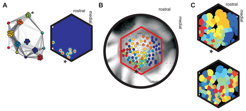
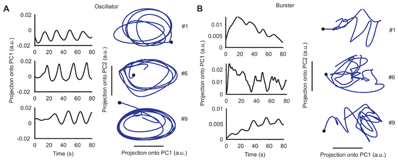
The neural substrates of motor programs are only well understood for small, dedicated circuits. Here we investigate how a motor program is constructed within a large network. We imaged populations of neurons in the Aplysia pedal ganglion during execution of a locomotion motor program. We found that the program was built from a very small number of dynamical building blocks, including both neural ensembles and low-dimensional rotational dynamics. These map onto physically discrete regions of the ganglion, so that the motor program has a corresponding modular organization in both dynamical and physical space. Using this dynamic map, we identify the population potentially implementing the rhythmic pattern generator and find that its activity physically traces a looped trajectory, recapitulating its low-dimensional rotational dynamics. Our results suggest that, even in simple invertebrates, neural motor programs are implemented by large, distributed networks containing multiple dynamical systems.

Figure 1. Imaging and analyzing Aplysia’s locomotion motor program.

A Experimental setup. Left: Head reach in Aplysia’s rhythmic escape locomotion. Middle: Preparations consisted of the ring ganglia (Ce: cerebral; Pl: pleural; Pd: pedal), with a stimulating electrode connected to peripheral nerve Pd9. Some recordings also used a suction electrode connected to pedal nerve 10 (Pd10) to monitor the neck contraction phase of locomotion. Right: Imaged area of the dorsal pedal ganglion, aligned to the photodiode array of 464 diodes (red outline). B Analysis stages for deconstructing the motor program. Fast voltage-sensitive dye recordings captured simultaneous cellular-level activity and the location of every neuron. Step 1: each motor program recording is decomposed into its component ensembles using modularity-detection (panel C). We map the physical location of the ensembles in each recording, seeking a “dynamic map” of each execution of the program. Step 2: ensembles are classified across recordings into groups of statistically similar firing patterns, seeking the dynamical building blocks of the motor program. Step 3: we map the physical location of the ensemble groups over all recordings, seeking the physical layout of the motor program’s dynamical building blocks. C Modularity detection of ensembles (step 1 in panel B). Schematic illustration of the steps for decoding neural ensembles using community detection with consensus clustering. Key is modelling the pairwise correlation matrix as a network: each node is a neuron, each link’s weight is the correlation between that pair of neurons. Community detection algorithms – so-called by analogy with the division of social networks into communities – provide a general solution to the problem of separating an arbitrary network into its component modules: here each module is thus an ensemble of strongly, mutually correlated neurons. Choice of time-scale and type of correlation thus define a “neural ensemble”. Here we convolve each spike-train with a Gaussian window whose width is defined by the characteristic period of the locomotion-related activity (Experimental Procedures; Supplemental Fig. 1), and correlate each pair of convolved spike-trains.

Figure 2. Modular deconstruction of a motor program recording.

A Raster plot of an example optical recording of 102 neurons over 80 seconds. B The corresponding functional network. Each node is a neuron; gray-scale intensity of the links indicates similarity of that pair of neurons. The 12 detected modules within the network are color-coded. Distance between modules indicates their average similarity. C Raster plot from panel A ordered and color coded by module membership in panel B, showing the 12 ensembles. D Distribution of ensemble size across all recordings. Red line indicates median value. E Distribution of median intra-group similarity over all preparations; red line indicates median of distribution. F Correlation between number of neurons in each recording and number of ensembles detected (linear regression, n = 12). (see also Supplemental Fig. 2).

Figure 3. Modular deconstruction of the physical substrate.

A Mapping neuron location. Left: layout of a recorded functional network; the asterisk (∗) indicates the example neural ensemble corresponding to physical positions in panels A-C. Right: Estimated position of all 8 neurons in the example ensemble; each position estimate is plotted as a two-dimensional Gaussian, with blue-red indicating minimum-maximum probability of location. B Projection of the functional network onto physical space. We plot the mean estimated position of all neurons, color-coded by ensemble membership, onto the approximate extent of the ganglion covered in this recording. Links show a sample of the network (within ± 1 s.d. of mean correlation). C Map of neural ensemble locations on the photodiode array (top) showing physical contiguity of the ensembles in a recording: each region of the array is claimed by the closest neuron; all regions belonging to the same neural ensemble are merged (same color). Bottom: example control map, generated by randomly assigning neurons to the same number and size of neural ensembles. Supplemental Figure 3 compares data and randomized maps across all recordings.

Figure 4. Classes of ensemble.

Four classes of ensemble were defined by the presence or absence of significant peaks or troughs in their auto-correlograms: the non-oscillatory class had no significant peaks or troughs; “oscillators” had both; “bursters” had significant peaks but not troughs, indicating repeated phasic firing without repeated silence; “pausers” had significant troughs but not peaks, indicating repeated silence without repeated stereotyped bursts. Auto-correlogram (top) and raster (bottom) plotted for an example ensemble of each class. The red lines plot the upper and lower bounds on expected spike-count predicted by a shuffled inter-spike interval model; peaks are contiguous bins above the upper bound, troughs are contiguous bins below the lower bound. We also plot the “dynamic map” of each oscillatory class, with heat intensity (blue-red) indicating the proportion (%) of recordings in which that location belonged to that oscillatory class of ensemble; white indicates no membership of that class detected. All maps plotted for the left ganglion.

Figure 5. Separate dynamical systems within the locomotion motor program.

A Oscillator-class ensembles. We plot the projection onto the first principal component (PC1, left) and onto the first two PCs (right) for the population of neurons in oscillator-class ensembles in three recordings (1, 6, and 9). Black dot indicates time zero. B Burster-class ensembles. Layout as for panel A, plotted for the population of neurons in burster-class ensembles in the same three recordings.

Figure 6. Rotational dynamics correspond to physical rotations of activity.

A Projection of oscillator-class activity onto physical space. Top: Sequence of firing of 4 representative oscillator ensembles in recording #1. Bottom: center of each of the 4 ensembles. Eligible recordings had 5-12 oscillator ensembles. B Looped trajectories of the activity packet in space. Top: the activity packet from recording #1 (panel A) describes an elliptical orbit (red) on the plane of the ganglion; black line: best-fit ellipse; scale bar: 1 diode spacing (∼ 60µm). Bottom: best-fit ellipses showing trajectories from all recordings with sufficient oscillator ensembles to uniformly span phases of a motor program cycle. C Looped trajectory corresponds to phasic motor output. Top: Extracellular recording from pedal nerve 10 (Pd10). Bottom: firing of Pd10 mapped onto the looped trajectory. Dark red represents peak firing, corresponding to bursts in the upper panel (see Supplemental Fig. 5). D Hypothesised control of the pedal wave for locomotion. Cycling activity on the network is plotted schematically as an ellipse. Activity on specific portions of the trajectory is proposed to recruit motorneurons (M) projecting to muscles in the foot and body wall, whose axons contribute to the suggested nerves. One cycle of the trajectory would thus generate the pedal wave for locomotion by sequentially activating the neck/anterior, middle, then posterior nerves.

Figure 7. Unsupervised clustering of ensembles in the “fit-space”.

A Ensemble characterization. Histograms show ISI or CV₂ distributions for three example ensembles, and red lines plot their best-fit models. A distribution for an ensemble was created by pooling distributions for each spike-train in the ensemble. B Clustering ensemble groups by spike-train structure. Top-left we plot two examples of concatenated P(model) vectors defining the 12-dimensional “fit-space”. Bottom-right: visualization of the network defined by distances between ensembles in this fit-space, and the nine identified ensemble-groups within it (colors); symbols indicate some common properties of the nine groups. Grayscale intensity of lines indicates similarity of nodes.

Figure 8. Groups of ensembles defined by spike-train structure.

We found nine groups of ensemble distinguished by their firing rate and regularity; percentages on the far left give the proportion of ensembles in each group. In the left-most column we plot the map of all locations containing that ensemble group, with heat intensity (blue-red) indicating the proportion of recordings in which that location contained an ensemble of that group; white indicates no membership of that group detected. Further columns illustrate an example ensemble of each group: the four most-similar spike-trains in that ensemble (80 s duration); and the cumulative distributions for the interspike intervals (ISIs) and the irregularity metric (CV₂) for the ensemble. Black line: data; red line: best fitting model (highest P(model) out of the 6 candidates). Note different scaling of x-axes for cumulative plots. Supplemental Figure 6 maps these ensemble groups defined by spike-train structure onto the distribution of ensembles according to oscillator-class.

References

1. Ahrens MB, Li JM, Orger MB, Robson DN, Schier AF, Engert F, Portugues R. Brain-wide neuronal dynamics during motor adaptation in zebrafish. Nature. 2012;485:471–477. - PMC - PubMed
1. Ahrens MB, Orger MB, Robson DN, Li JM, Keller PJ. Whole-brain functional imaging at cellular resolution using light-sheet microscopy. Nat Methods. 2013;10:413–420. - PubMed
1. Berg RW, Alaburda A, Hounsgaard J. Balanced inhibition and excitation drive spike activity in spinal half-centers. Science. 2007;315:390–393. - PubMed
1. Brezina V, Orekhova IV, Weiss KR. The neuromuscular transform: the dynamic, nonlinear link between motor neuron firing patterns and muscle contraction in rhythmic behaviors. J Neurophysiol. 2000;83:207–231. - PubMed
1. Briggman KL, Abarbanel HDI, Kristan W., Jr Optical imaging of neuronal populations during decision-making. Science. 2005;307:896–901. - PubMed
Publication types
LinkOut - more resources