Coil combination for receive array spectroscopy: Are data-driven methods superior to methods using computed field maps?

Abstract

Purpose: Combining spectra from receive arrays, particularly X-nuclear spectra with low signal-to-noise ratios (SNRs), is challenging. We test whether data-driven combination methods are better than using computed coil sensitivities.

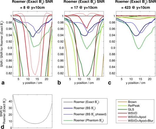
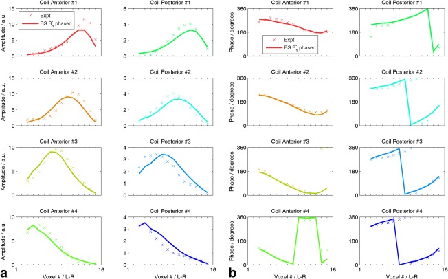
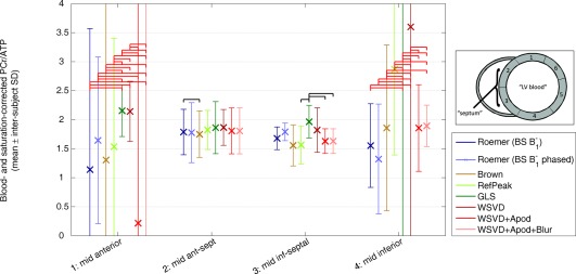
Theory: Several combination algorithms are recast into the notation of Roemer's classic formula, showing that they differ primarily in their estimation of coil receive sensitivities. This viewpoint reveals two extensions of the whitened singular-value decomposition (WSVD) algorithm, using temporal or temporal + spatial apodization to improve the coil sensitivities, and thus the combined spectral SNR.

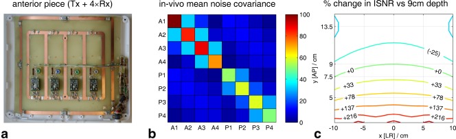
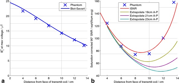
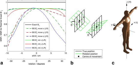
Methods: Radiofrequency fields from an array were simulated and used to make synthetic spectra. These were combined with 10 algorithms. The combined spectra were then assessed in terms of their SNR. Validation used phantoms and cardiac (31) P spectra from five subjects at 3T.

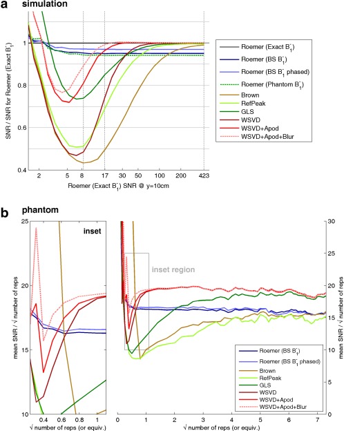
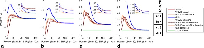
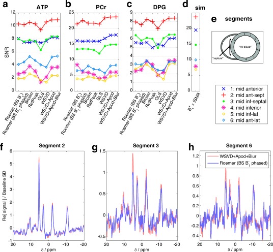
Results: Combined spectral SNRs from simulations, phantoms, and humans showed the same trends. In phantoms, the combined SNR using computed coil sensitivities was lower than with WSVD combination whenever the WSVD SNR was >14 (or >11 with temporal apodization, or >9 with temporal + spatial apodization). These new apodized WSVD methods gave higher SNRs than other data-driven methods.

Conclusion: In the human torso, at frequencies ≥49 MHz, data-driven combination is preferable to using computed coil sensitivities. Magn Reson, 2015. © 2015 The Authors. Magnetic Resonance in Medicine published by Wiley Periodicals, Inc. on behalf of International Society for Magnetic Resonance in Medicine. This is an open access article under the terms of the Creative Commons Attribution License, which permits use, distribution and reproduction in any medium, provided the original work is properly cited. Magn Reson Med 75:473-487, 2016. © 2015 The Authors. Magnetic Resonance in Medicine published by Wiley Periodicals, Inc. on behalf of International Society for Magnetic Resonance in Medicine.

Keywords: MR spectroscopy; WSVD; WSVD+Apod; WSVD+Apod+Blur; adaptive combination theory; array; coil combination.

Figure 1

(a) Photograph of the anterior half of the eight‐element cardiac ³¹P 3T receive array coil employed in study. (b) Noise covariance matrix for this array. (Diagonal elements of the noise covariance matrix are the single‐coil noise variances. Note that this is not the same as the noise correlation matrix whose diagonal elements are all equal to 1 24.) (c) Contour plot of ISNR 24 in the midtransverse plane for the receive array with a 27‐cm separation between conducting elements. This plot is scaled relative to the interventricular septum (9‐cm depth). Horizontal lines mark the mean depth of the anterior mid‐short axis segments (7.5‐cm depth) and the inferior mid‐short axis segments (13.5 cm) across all subjects. A, anterior; ISNR, intrinsic signal‐to‐noise ratio; LR, left–right; P, posterior.

Figure 2

Validation of transmit and receive fields computed using the Biot‐Savart law against single‐depth experimental values from the phantom in Supporting Figure S1. (a) B₁ ⁺ profile. Line shows B₁ ⁺ computed using the Biot‐Savart law and nonlocalized inversion recovery data from the anterior fiducial. Each experimental value (x) is obtained by fitting a sinusoid to a series of fully relaxed, nonlocalized FIDs, with increasing flip angles acquired with the phosphate cube at that depth. (b) Experimental points show WSVD‐combined signal amplitude for fully‐relaxed 90° excitation at each depth. Red line shows corresponding ISNR values 24 computed at experimental coil separation (16.7 cm) and scaled vertically to fit experimental data. Other lines extrapolate experimental signals to model greater separations between anterior and posterior pieces of the array, which would be more representative of human subjects. AP, anterior–posterior; ISNR, intrinsic signal‐to‐noise ratio; WSVD, whitened singular value decomposition.

Figure 3

Performance of different coil combination algorithms applied to simulated spectra. The simulated receive array has 4× elements in the plane at y = 0 cm and 4× elements in the plane at y = 25 cm. Coordinate system is shown in Figure 5c; y is anterior‐posterior direction. (a–c) Mean SNR along a column from x = −10 to +10 cm at different depths. Values are plotted relative to SNR for Roemer (Exact B₁ ⁻) combination. (d) Spatial variation of mean SNR for Roemer (Exact B₁ ⁻) combination. Apod, apodized; BS, Biot‐Savart law; GLS, generalized least squares; SNR, signal‐to‐noise ratio; WSVD, whitened singular value decomposition.

Figure 4

Summary of coil combination performance as a function of SNR. (a) Simulation. Each point on a line shows the mean over a 20 cm‐ (L–R) × 5‐cm (AP) region centered at 10‐cm depth (i.e., at the interventricular septum) of the SNR relative to the SNR for Roemer (Exact B₁ ⁻) combination. Gray vertical lines mark the three SNR levels detailed in Figures 3a–c. (b) Phantom. Coil combination performance as a function of SNR in a uniform KH₂PO_4(aq) phantom. Raw data comprise 54 three‐dimensional ultrashort echo‐time chemical‐shift imaging acquisitions. These were averaged in bunches to yield effective single‐element data with different SNRs, which were then combined. To better characterize the low‐SNR regime, further noise with the experimental covariance matrix was added before combination to give values with < 1 “repetitions”. Inset. Expanded view for low SNR. AP, anterior–posterior; Apod, apodized; BS, Biot‐Savart law; GLS, generalized least squares; LR, left–right; SNR, signal‐to‐noise ratio; WSVD, whitened singular value decomposition.

Figure 5

Sensitivity of Roemer (BS B₁ ⁻) combination to misalignment of the coil relative to its expected location or orientation. For each point plotted, anterior and posterior pieces of the array were either translated by an equal and opposite amount parallel to the specified axis or rotated around the center of each piece by an equal and opposite angle around the specified axis. No noise was added during these calculations, that is, this figure corresponds to the high SNR limit at the right‐hand edge of Figure 4a. (a) Mean SNR relative to SNR for Roemer (Exact B₁ ⁻) combination. (b) Diagram showing coil geometry for the “rot x” case. (c) Coordinate system employed 65. BS, Biot‐Savart law; H, head; L, left; P, posterior; R, right; SNR, signal‐to‐noise ratio.

Figure 6

Simulation of coil combination performance in a two‐compartment phantom with a point spread function that gives 10% bleed from neighbouring voxels. Simulations were run 2000 times at each of 31 noise levels before averaging. Dotted lines show the effect of adding an extra 2% nonlocalized baseline “artifact” to the single‐element spectra before they are combined. Inset: Vertically magnified view of the same data for SNR from 40 to 400. Apod, apodized; GLS, generalized least squares; PCr/ATP, phosphocreatine to adenosine triphosphate concentration ratio; SNR, signal‐to‐noise ratio; WSVD, whitened singular value decomposition.

Figure 7

Illustration of phase/gain corrected B₁ ⁻ fields from the procedure in Appendix 1. (a) Amplitudes and (b) phases for voxels running L‐R along center of uniform phantom. AMARES fits to the phosphate resonance are denoted x and the singular value decomposition best‐fit calculated B₁ ⁻ is plotted with a line. BS, Biot‐Savart law; L‐R, left–right; AMARES, accurate, robust and efficient spectral fitting method.

Figure 8

Comparison of mean metabolite SNRs after application of different coil combination algorithms for five normal volunteers. (a–c) Points show mean metabolite SNRs (average of α‐ATP, β‐ATP, γ‐ATP peak SNRs, PCr SNR, and average of 2,3‐DPG peak SNRs) in each mid‐short axis myocardial segment for each coil combination algorithm. Lines are only to guide eye. (d) B₁ ⁺ × ISNR at the mean centroid of each segment. This value should be proportional to SNR in the limit of low flip angle and long repetition time. (e) Inset showing segment numbering 48. (f–h) Example spectra from a voxel in the centre of each segment combined with the best data‐driven and the best field map‐driven algorithms. Apod, apodized; BS, Biot‐Savart law; GLS, generalized least squares; PCr/ATP, phosphocreatine to adenosine triphosphate concentration ratio; DPG, 2,3‐diphosphoglycerate; SD, standard deviation; SNR, signal‐to‐noise ratio; WSVD, whitened singular value decomposition.

Figure 9

Comparison of blood‐ and saturation‐corrected PCr/ATP ratios for five normal volunteers. Points show intersubject mean metabolite ratio in each segment for each coil combination algorithm. Error bars show corresponding intersubject SD. Black horizontal bars indicate a statistically significant change in PCr/ATP ratio for different combination algorithms (i.e., P < 0.05 from a paired t test). Red horizontal bars indicate a statistically significant change in PCr/ATP variance (i.e., P < 0.05 from a paired two‐sample F test for equal variances). Apod, apodized; BS, Biot‐Savart law; GLS, generalized least squares; PCr/ATP, phosphocreatine to adenosine triphosphate concentration ratio; SD, standard deviation; WSVD, whitened singular value decomposition.

References

1. De Graaf RA. In vivo NMR Spectroscopy: Principles and Techniques. Chichester, UK: John Wiley & Sons; 2007. 570 p.
1. Tyler D. Cardiovascular applications of hyperpolarized MRI. Curr Cardiovasc Imaging Rep 2011; 4: 108–115. - PMC - PubMed
1. Bottomley PA. NMR Spectroscopy of the Human Heart In: Harris RK, Wasylishen RE, editors. Encyclopedia of Magnetic Resonance. Chichester, UK: John Wiley; 2009. doi 10.1002/9780470034590.emrstm0345.pub2. - DOI
1. Roemer PB, Edelstein WA, Hayes CE, Souza SP, Mueller OM. The NMR Phased Array. Magn Reson Med 1990; 16: 192–225. - PubMed
1. Wright SM, Wald LL. Theory and application of array coils in MR spectroscopy. NMR Biomed 1997; 10: 394–410. - PubMed