

Intermittency, nonlinear dynamics and dissipation in the solar wind and astrophysical plasmas
- PMID: 25848085
- PMCID: PMC4394684
- DOI: 10.1098/rsta.2014.0154
Intermittency, nonlinear dynamics and dissipation in the solar wind and astrophysical plasmas
Abstract
An overview is given of important properties of spatial and temporal intermittency, including evidence of its appearance in fluids, magnetofluids and plasmas, and its implications for understanding of heliospheric plasmas. Spatial intermittency is generally associated with formation of sharp gradients and coherent structures. The basic physics of structure generation is ideal, but when dissipation is present it is usually concentrated in regions of strong gradients. This essential feature of spatial intermittency in fluids has been shown recently to carry over to the realm of kinetic plasma, where the dissipation function is not known from first principles. Spatial structures produced in intermittent plasma influence dissipation, heating, and transport and acceleration of charged particles. Temporal intermittency can give rise to very long time correlations or a delayed approach to steady-state conditions, and has been associated with inverse cascade or quasi-inverse cascade systems, with possible implications for heliospheric prediction.
Keywords: intermittency; plasma physics; solar corona; solar wind; turbulence theory.
© 2015 The Author(s) Published by the Royal Society. All rights reserved.
Figures


 and
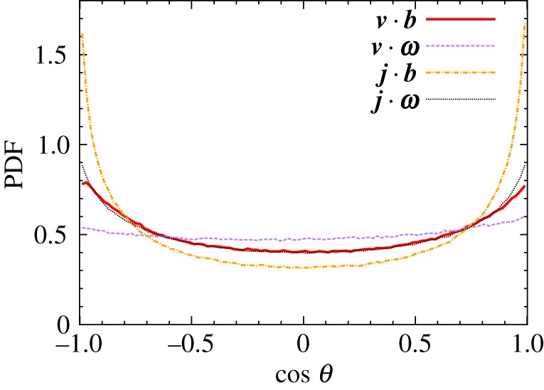
and  computed from solar wind (SW) data and from an MHD turbulence simulation initiated with the same dimensionless cross helicity as the solar wind sample. Simulation results are for a time a few nonlinear times from the initial data. The similarity may be viewed as evidence that the spatial patchiness of correlation seen in the simulations, necessarily associated with non-Gaussian distributions, also occurs in the solar wind. (From Osman et al. [82].) (Online version in colour.)


Similar articles
-
Dissipation and heating in solar wind turbulence: from the macro to the micro and back again.Philos Trans A Math Phys Eng Sci. 2015 May 13;373(2041):20140155. doi: 10.1098/rsta.2014.0155. Philos Trans A Math Phys Eng Sci. 2015. PMID: 25848077 Free PMC article.
-
Mediation of collisionless turbulent dissipation through cyclotron resonance.Nat Astron. 2024;8(4):482-490. doi: 10.1038/s41550-023-02186-4. Epub 2024 Jan 23. Nat Astron. 2024. PMID: 38659611 Free PMC article.
-
Detection of small-scale structures in the dissipation regime of solar-wind turbulence.Phys Rev Lett. 2012 Nov 9;109(19):191101. doi: 10.1103/PhysRevLett.109.191101. Epub 2012 Nov 8. Phys Rev Lett. 2012. PMID: 23215371
-
A dynamical model of plasma turbulence in the solar wind.Philos Trans A Math Phys Eng Sci. 2015 May 13;373(2041):20140145. doi: 10.1098/rsta.2014.0145. Philos Trans A Math Phys Eng Sci. 2015. PMID: 25848075 Free PMC article. Review.
-
Kinetic scale turbulence and dissipation in the solar wind: key observational results and future outlook.Philos Trans A Math Phys Eng Sci. 2015 May 13;373(2041):20140147. doi: 10.1098/rsta.2014.0147. Philos Trans A Math Phys Eng Sci. 2015. PMID: 25848084 Free PMC article. Review.
Cited by
-
Open-Source Software Analysis Tool to Investigate Space Plasma Turbulence and Nonlinear DYNamics (ODYN).Earth Space Sci. 2020 Apr;7(4):e2019EA001004. doi: 10.1029/2019EA001004. Epub 2020 Apr 22. Earth Space Sci. 2020. PMID: 32715025 Free PMC article.
-
Multifractal and Chaotic Properties of Solar Wind at MHD and Kinetic Domains: An Empirical Mode Decomposition Approach.Entropy (Basel). 2019 Mar 25;21(3):320. doi: 10.3390/e21030320. Entropy (Basel). 2019. PMID: 33267034 Free PMC article.
-
The role of turbulence in coronal heating and solar wind expansion.Philos Trans A Math Phys Eng Sci. 2015 May 13;373(2041):20140148. doi: 10.1098/rsta.2014.0148. Philos Trans A Math Phys Eng Sci. 2015. PMID: 25848083 Free PMC article. Review.
-
Magneto-immutable turbulence in weakly collisional plasmas.J Plasma Phys. 2019 Feb;85(1):905850114. doi: 10.1017/s0022377819000114. Epub 2019 Feb 18. J Plasma Phys. 2019. PMID: 35136272 Free PMC article.
-
Turbulent reconnection and its implications.Philos Trans A Math Phys Eng Sci. 2015 May 13;373(2041):20140144. doi: 10.1098/rsta.2014.0144. Philos Trans A Math Phys Eng Sci. 2015. PMID: 25848076 Free PMC article. Review.
References
-
- van Dyke M. 1982. An album of fluid motion. Stanford, CA: Parabolic Press.
-
- Samimy M, Breuer KS, Leal LG, Steen H. 2003. A gallery of fluid motion. Cambridge, UK: Cambridge University Press.
-
- Novikov EA. 1971. Intermittency and scale similarity in the structure of a turbulent flow. J. Appl. Math. Mech. 35, 231–241. (10.1016/0021-8928(71)90029-3) - DOI
-
- Oboukhov AM. 1962. Some specific features of atmospheric turbulence. J. Fluid Mech. 13, 77–81. (10.1017/S0022112062000506) - DOI
-
- Kolmogorov AN. 1962. A refinement of previous hypotheses concerning the local structure of turbulence in a viscous incompressible fluid at high Reynolds number. J. Fluid Mech. 13, 82–85. (10.1017/S0022112062000518) - DOI
Publication types
LinkOut - more resources
Full Text Sources
Other Literature Sources
