Diverse coupling of neurons to populations in sensory cortex

Abstract

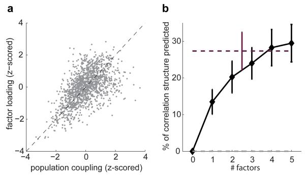
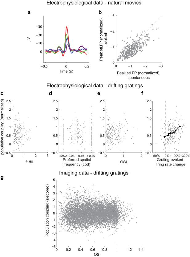
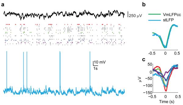
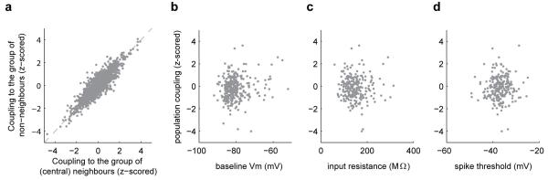
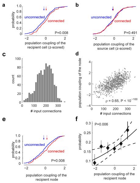
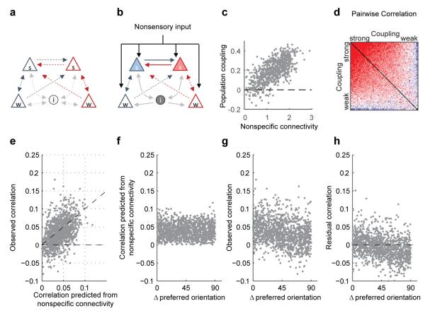
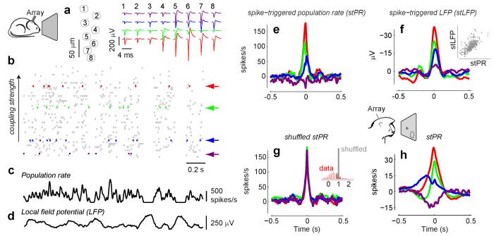
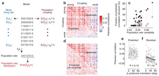
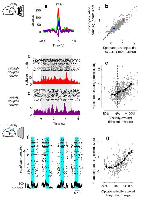
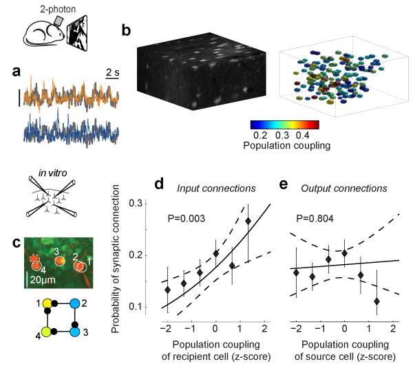
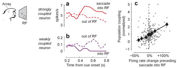
A large population of neurons can, in principle, produce an astronomical number of distinct firing patterns. In cortex, however, these patterns lie in a space of lower dimension, as if individual neurons were "obedient members of a huge orchestra". Here we use recordings from the visual cortex of mouse (Mus musculus) and monkey (Macaca mulatta) to investigate the relationship between individual neurons and the population, and to establish the underlying circuit mechanisms. We show that neighbouring neurons can differ in their coupling to the overall firing of the population, ranging from strongly coupled 'choristers' to weakly coupled 'soloists'. Population coupling is largely independent of sensory preferences, and it is a fixed cellular attribute, invariant to stimulus conditions. Neurons with high population coupling are more strongly affected by non-sensory behavioural variables such as motor intention. Population coupling reflects a causal relationship, predicting the response of a neuron to optogenetically driven increases in local activity. Moreover, population coupling indicates synaptic connectivity; the population coupling of a neuron, measured in vivo, predicted subsequent in vitro estimates of the number of synapses received from its neighbours. Finally, population coupling provides a compact summary of population activity; knowledge of the population couplings of n neurons predicts a substantial portion of their n(2) pairwise correlations. Population coupling therefore represents a novel, simple measure that characterizes the relationship of each neuron to a larger population, explaining seemingly complex network firing patterns in terms of basic circuit variables.

Extended Data Figure 1. Pearson correlation between spike trains of individual units and the population rate

To estimate the relation of a neuron to the population, an alternative to stPR would have been to compute the Pearson correlation coefficient of the the neuron’s spike train with the summed population rate of all other recorded cells (a measure we term “Pearson coupling”). This measure, however, is biased by firing rate. a, Pearson coupling and stPR were computed for a set of individual units in an example experiment. Pearson coupling is related to the stPR, but not identical to it. b, The numerical value of the Pearson coupling depends strongly on the bin size used, but the correlations measured with different bin size are tightly related. c, Pearson correlation is biased by firing rate^,. The spike train of a single cell was “thinned” to different firing rates by keeping only a random subset of its spikes; Pearson correlation with the population was recalculated for different values of firing rate. A strong effect of firing rate is seen. d, Performing the same analysis for population coupling (measured by stPR) demonstrates that this measure does not suffer from rate bias. For this reason, we chose to quantify population coupling with stPR in this work.

Extended Data Figure 2. Neighbouring neurons differ markedly in population coupling during spontaneous activity

a, Dividing the data into two halves shows that population coupling, measured as the height of stPR at 0 time lag, is highly consistent over time (n=431 neurons from 13 experiments; ρ=0.76, P<10⁻¹⁰⁰, rank correlation). Coloured dots represent the four example cells. b, As in a for peak stLFP (ρ=0.58, P<10⁻⁹). c, Differences in stLFP disappear after shuffling spikes in a manner that preserves each neuron’s mean firing rate and the population rate (cf. Fig. 1g). Inset: stLFPs in the actual spike trains (red) and after shuffling (gray), for neurons from all experiments (cf. Fig. 1g). d, stPR size of V4 neurons is consistent over time (n=262 neurons from 43 experiments; ρ=0.95, P<10⁻¹⁰⁰, rank correlation).

Extended Data Figure 3. Neighbouring neurons in auditory cortex differ markedly in population coupling

a, Spike-triggered population rate (stPR) for four example neurons recorded on the same electrode shank, during spontaneous activity in rat primary auditory cortex. b, Differences in population coupling disappear after shuffling spikes in a manner that preserves each neuron’s mean firing rate and the population rate distribution. c,d As in (a,b) for the spike-triggered local field potential (stLFP). e, Dividing the data into two halves shows that population coupling, measured as the height of stPR at 0 time lag, is highly consistent over time (n=76 neurons from 3 experiments; ρ=0.92, P<10⁻¹⁰⁰, rank correlation). Colored dots represent the four example cells. f, As in e, for stLFP (ρ=0.81, P<10⁻¹⁰⁰, rank correlation).

Extended Data Figure 4. Firing rate, burstiness and population coupling

a, Similarly to other studies^, our recordings allow separation of narrow spiking (putative Pvalb+ inhibitory) and wide spiking (primarily excitatory pyramidal) neurons. Here, we used a trough to peak time of 0.66 ms as the separation criterion. b, There is a negative correlation between burstiness (the ratio between the peak and baseline of a neuron’s autocorrelogram) and mean firing rate, which is also the case individually for wide spiking (n=384, ρ=−0.60, P<10⁻⁹, rank correlation) and narrow spiking (n=47, ρ=−0.82, P<10⁻⁹, rank correlation) neurons. c, There is a positive correlation between burstiness and population coupling, which is also the case individually for wide spiking (ρ=0.46, P<10⁻⁹, rank correlation) and narrow spiking (ρ=0.50, P=4·10⁻⁴, rank correlation) neurons. d, There is a negative correlation between firing rate and population coupling, which is also the case individually for wide spiking (ρ=−0.27, P=10⁻⁷, rank correlation) and narrow spiking (ρ=−0.37, P=0.01, rank correlation) neurons. The correlation between population coupling and firing rate can be predicted from the correlations between burstiness and firing rate and between population coupling and burstiness: the partial rank sum correlation between population coupling and firing rate, once burstiness is taken into account, is insignificant (ρ=0.06, P=0.25). This is also the case for wide spiking (ρ=0.01, P=0.78) and narrow spiking (ρ=0.07, P=0.65) neurons individually.

Extended Data Figure 5. Latent variable analysis

a, Population coupling of each neuron is highly correlated with its loading in a single-factor latent variable model (see Methods). The similarity of each cell’s population coupling and loading indicates that the low-dimensional structure found by the latent variable model is homologous to that found by the coupling model. b, Percent of pairwise correlation structure explained by a latent variable model with 1-5 factors (black), and by the coupling model introduced in the present study (dashed purple line). Error bars show S. E. While the coupling model outperforms latent variable models with less than four degrees of freedom, this difference may arise primarily from the assumption of a Gaussian distribution for the latent variables. Indeed, if the population rate distribution generated by the latent variable model is substituted into the coupling model instead of the (correct) populate rate distribution, extremely poor performance results (dashed grey line; almost on top of the x-axis).

Extended Data Figure 6. Population coupling and visual stimulation in mouse V1

a, stLFPs computed for the four example neurons of Fig. 1a-f, from intervals of natural movie presentation (inverted for ease of comparison, cf. Fig. 1f). b, Comparison of stLFP size during spontaneous and evoked activity across all experiments (ρ=0.72, P<10⁻¹⁰⁰, rank correlation). c-e, Population coupling is plotted vs. the f1/f0 ratio, preferred spatial frequency and orientation selectivity index (OSI) for neurons recorded in the infragranular layers of V1. All correlations are statistically insignificant. f, Similar to movie presentations (cf. Fig. 3e), the mean change in the activity of a cell in response to grating presentations (relative to baseline, averaged across contrasts and orientations) correlates with population coupling measured during spontaneous activity (ρ=0.32, P=2*10⁻⁶, n=217, rank correlation). Black diamonds: running median. g, In the 2-photon imaging data (of ~10,000 cells) only a very weak correlation between OSI and population coupling was found (ρ=0.066, P<10⁻⁹, rank correlation).

Extended Data Figure 7. stLFP reflects the correlation between membrane potential (Vm) and LFP

a, Example of a silicon probe population recording performed simultaneously with a whole-cell recording (in an anaesthetised animal). Four neurons shown in colour were recorded on the same shank of the silicon probe. b, Comparison of stLFP and Vm-LFP crosscorrelation (VmLFPcc, appropriately scaled along the ordinate axis) for the intracellularly recorded cell. c, stLFP for the four neurons from a and the intracellularly recorded neuron, exhibiting diversity in the strength of coupling to LFP.

Extended Data Figure 8. Population coupling in 2-photon data is not correlated with location and intrinsic properties of the neurons

a, For each neuron in the central region of the imaging field (defined as a square 1/4 of the total imaging area), we compared its coupling to the population of all other neurons in the central region, with its coupling to population of all neurons outside of the central region. The two were highly similar; this was the case because the two population rate signals were themselves highly correlated (on average across experiments the Pearson correlation was 0.77). Thus, differences in population coupling measured between cells do not reflect differences in the fraction of nearby neurons imaged. b-d, No significant correlation was observed between population coupling (measured in vivo) and resting potential, input resistance and spike threshold (subsequently measured in vitro).

Extended Data Figure 9. Correlation between input connectivity and population coupling

a, Cumulative distribution of population coupling of a target pyramidal neuron when an input connection was present (red) and when it was absent (blue). The medians (arrows) are significantly different. b, As in a, for population coupling of the source pyramidal cells. (The distributions shown were used for the logistic regression analysis in Fig. 4). c-f, We constructed random directed graphs of 1000 nodes (each node representing a L2/3 pyramidal cell) with the probability of connection from node j to node i given by $\sqrt{p_{in}^i{p}_{out}^j}$, where the propensities to receive and provide connections (p_in and p_out, correspondingly) were randomly and independently chosen for each node from a Gaussian distribution. The resulting distribution of the number of input connections in a typical network is shown in c; the number of output connections was (by construction) similarly distributed. In addition, each node was assigned a population coupling value, highly correlated to the number of its input connections (on average ρ=0.65); this correlation in a typical network is shown in d. We next asked how the relationship between measured connectivity and population coupling would look if we sample from 33 such randomly generated networks (equal to the number of animals used in our experimental data), the same amount of data empirically available in our in vitro recordings (i.e., the connections between 2-3 randomly selected groups of 2-6 nodes). Results very similar to those of Fig. 4 were typically obtained (e,f; cf. a and Fig. 4d; error bars in f indicate standard error for binned data). In particular, when the entire procedure was repeated 1000 times, in over 30% of the cases the P-value of the difference between the medians (presented in a,e) was higher (i.e., less statistically significant) than the value of 0.008 obtained in the actual data. Thus, the results shown in Fig. 4 and in a are consistent with a strong correlation between connection probability and population coupling.

Extended Data Figure 10. Mathematical model for the relationship between nonspecific connectivity, specific connectivity, and correlations

a, A recurrent network where excitatory cells (triangles) send synaptic connections (arrows) to each other and to inhibitory cells (circles). Weakly coupled neurons (bottom) receive only connections from neurons with similar sensory preference (e.g. for stimulus orientation, indicated in blue vs. red). Strongly coupled neurons (top) also receive nonspecific connections from neurons of different sensory preference. b, The effect of nonspecific drive, such as caused by non-sensory top-down inputs, or occurring due to artificial optogenetic stimulation, is amplified through recurrent connections, leading to stronger activation of neurons with greater mean local input (darker shading). c,d correlations predicted by the model (analytically derived in Supplementary Information): c - population coupling vs. nonspecific connectivity c_i, for all simulated excitatory neurons. d - pseudocolor plot of predicted pairwise correlations for a random subset of excitatory neurons, ordered by population coupling. e-h, dependence of correlations on specific and nonspecific connectivity. e - predicted correlations based on nonspecific connections vs total observed correlations. f - predicted correlation based on nonspecific connectivity vs. difference in preferred orientation. As in the experimental data (Fig. 2e), no relation is observed. g - observed correlation vs difference in preferred orientation. As has been widely reported, observed correlations are largest for neurons of similar orientation preference. h - residual correlation (after removing prediction from nonspecific connectivity) vs difference in preferred orientation. Again as in our experimental data (Fig. 2f), the residual correlation is largest for neurons of similar orientation preference, indicating an additive relationship between correlations generated by specific connections and correlations generated by nonspecific connections.

Figure 1. Neighbouring neurons differ markedly in population coupling during spontaneous activity

a, Schematic of a single shank of silicon electrode array, and spike waveforms of four example wide-spiking neighbour neurons measured with the array in deep layers of V1 of an awake mouse. b, Population raster of spontaneous activity in 66 neurons recorded from the whole array. Cells are arranged vertically in order of population coupling. Arrows indicate the four example neurons shown in a. c, Population rate measured by summing all the spikes detected on the entire array. d, Local field potential (LFP) measured on a shank adjacent to that on which the example neurons were recorded (LFP waveforms were similar across shanks). e, Spike-triggered population rate (stPR) for the four example neurons. The spike train of each neuron was excluded from the population rate before computing its stPR. f, The spike-triggered local field potential (stLFP) for the four example cells (inverted for ease of comparison) resembles their stPR (shown in e). Inset: normalised magnitudes of stPR and stLFP (see Methods) are highly correlated across cells (ρ=-0.71, P<10⁻¹⁰⁰, rank correlation, n=431 neurons). g, Differences in population coupling disappear after shuffling spikes in a manner that preserves each neuron’s mean firing rate and the population rate. Inset: population couplings in the actual spike trains (red) and after shuffling (grey), for neurons from all experiments. h, stPR of four example neurons simultaneously recorded in primate area V4, computed as in e.

Figure 2. A simple model based on population coupling predicts the structure of pairwise correlations in a cortical population

a, The model generates random spike patterns subject to three constraints: that the population coupling of each neuron, the mean firing rate of each neuron, and the distribution of the population rate, must match those in the original data. b, Random activity generated by the model produces pairwise correlations that are similar to those measured in the original spike trains (n=67 units in one experiment; correlations computed in 20ms bins). The upper triangle shows observed pairwise correlations, and the lower one shows pairwise correlations predicted by the model. Neurons are arranged in order of population coupling (arrows). The values on the diagonal (all 1s) have been removed. Similarity of observed and predicted correlations is indicated by the symmetry of the upper and lower triangles. c, Percentage of explainable correlation structure predicted, as a function of the variability of population rate (filled symbols, see Methods). The model captures pairwise correlations, but only in experiments in which the population rate fluctuates. It cannot predict them when population rate is mostly constant (a highly desynchronised cortical state). Recordings were obtained from mouse V1 in wakefulness (diamonds) or under anaesthesia (circles), or from A1 of awake rat (squares), all spontaneous activity; note that a variety of states is observed in all conditions. Open symbols show predictions of model that ignores population coupling. The example experiment in b is shown in red. d, Same as b, for predictions made without using population coupling. Such predictions fail to capture the structure of pairwise correlations (open markers in c). e, The model cannot predict a relationship between similarity of preferred orientation and spontaneous pairwise correlations (P=0.15, Pearson correlation). f, As a result, this correlation is retained in the residual pairwise correlations obtained by subtracting the modelled from actual correlations (ρ=0.26, P<10⁻³, Pearson correlation), indicating that the predictions of coupling and orientation sum linearly. The black line in f shows regression on cos(2Δθ).

Figure 3. Population coupling under natural and optogenetic stimulation conditions

a, Spike-triggered population rate (stPR) for the four example neurons in Fig. 1a-h during responses to a natural movie. The curves are similar to those measured during spontaneous activity (Fig. 1e). b, Comparison of population coupling during spontaneous and evoked activity, across cells and experiments (ρ=0.88, P<10⁻¹⁰⁰, rank correlation). c, Spike rasters (one row per presentation of a natural movie) and corresponding firing rate for a strongly coupled neuron (red neuron in a). Dashed line indicates baseline firing rate. d, Same, for a weakly coupled neuron (purple neuron in a). e, The increase in mean firing rate of a cell in response to natural movie presentations (relative to baseline) correlates with population coupling measured during spontaneous activity (ρ=0.38, P<10⁻¹⁵, rank correlation, n=431 neurons from 13 recordings in 8 animals). Black diamonds: running median. Points outside the x-axis range appear at the border for display purposes. f, Population rasters showing activity of deep-layer V1 neurons during four example trials (out of 75 in total), where the network was optogenetically driven by blue light in a mouse expressing Channelrhodopsin-2 sparsely in layer 5. Neurons are sorted by their population coupling during spontaneous activity. g, Change in mean firing rate evoked by optogenetic stimulation correlates with population coupling measured during spontaneous activity (ρ=0.51, P<10⁻¹⁰⁰, rank correlation, n=237 neurons). Points outside the x-axis range appear at the border for display purposes.

Figure 4. Neurons with strong population coupling receive more synaptic inputs from their neighbours

a, Neurons in superficial layers of mouse V1 were bulk-loaded with OGB-1 and their activity recorded using 2-photon imaging during presentation of natural movies and images. Population coupling was assessed as the correlation between each cell’s calcium signal with the summed signal of all other neurons. The two coloured traces show a segment of activity from a strongly and a weakly coupled neuron (orange and blue), each superimposed on the averaged population activity (gray). Scalebar: 20% ΔF/F for each single neuron, 5% for population average. b, Left, structural scan of an imaged volume measuring ~260×260×56 μm. Right, pseudocolour representation of population coupling for each of 147 neurons in the volume. c, Synaptic connectivity of a subset of the imaged neurons was later assessed using simultaneous in vitro whole-cell recordings. Top, four example pyramidal cells (solid white circles), recorded in vitro together with an additional fast-spiking interneuron (dashed circle) that was excluded from later analysis. Bottom, four synaptic connections were found between these 4 pyramidal neurons, shown here coloured by their in vivo population coupling. The two weakly coupled neurons (blue) received 0 or 1 inputs, while the strongly coupled neuron (yellow) received two inputs. d, Logistic regression estimate of probability to receive a synaptic connection as a function of the population coupling of the target (dashed black lines: 95% confidence intervals, error bars: mean and S.E. for binned data). e, As in d, for outgoing connections.

Figure 5. Population coupling under top-down stimulation conditions

a, Mean firing rate of an example neuron in primate V4 with strong population coupling (red neuron in Fig. 1h). This neuron showed higher firing rate (solid curve) while saccades were prepared into its receptive field (RF) than outside of it (dashed curve). b, An example neuron with weak population coupling (purple neuron in Fig. 1h) showed suppressed firing during saccade preparation into its RF. c, The change in firing rate of V4 neurons during saccade preparation into their RF (relative to saccade out of their RF) correlates with population coupling (ρ=0.37, P=10⁻⁹, rank correlation, n=262 neurons). Black diamonds: running median.

References

1. Tsodyks M, Kenet T, Grinvald A, Arieli A. Linking spontaneous activity of single cortical neurons and the underlying functional architecture. Science. 1999;286:1943–1946. - PubMed
1. Yu BM, et al. Gaussian-process factor analysis for low-dimensional single-trial analysis of neural population activity. Journal of neurophysiology. 2009;102:614–635. - PMC - PubMed
1. Luczak A, Bartho P, Harris KD. Spontaneous events outline the realm of possible sensory responses in neocortical populations. Neuron. 2009;62:413–425. - PMC - PubMed
1. Pfau D, Pnevmatikakis EA, Paninski L. Advances in Neural Information Processing Systems. :2391–2399.
1. Kenet T, Arieli A, Tsodyks M, Grinvald A. In: 23 Problems in Systems Neuroscience. van Hemmen JL, Sejnowski TJ, editors. Oxford University Press; 2006. Ch. 9.
Publication types