Cellular level brain imaging in behaving mammals: an engineering approach

Abstract

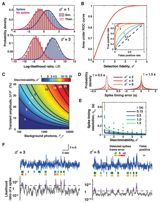
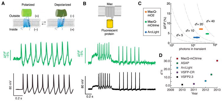
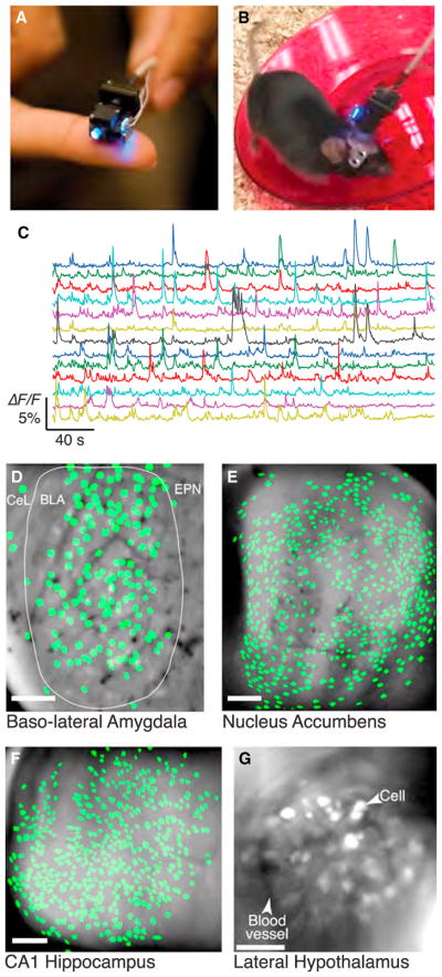
Fluorescence imaging offers expanding capabilities for recording neural dynamics in behaving mammals, including the means to monitor hundreds of cells targeted by genetic type or connectivity, track cells over weeks, densely sample neurons within local microcircuits, study cells too inactive to isolate in extracellular electrical recordings, and visualize activity in dendrites, axons, or dendritic spines. We discuss recent progress and future directions for imaging in behaving mammals from a systems engineering perspective, which seeks holistic consideration of fluorescent indicators, optical instrumentation, and computational analyses. Today, genetically encoded indicators of neural Ca(2+) dynamics are widely used, and those of trans-membrane voltage are rapidly improving. Two complementary imaging paradigms involve conventional microscopes for studying head-restrained animals and head-mounted miniature microscopes for imaging in freely behaving animals. Overall, the field has attained sufficient sophistication that increased cooperation between those designing new indicators, light sources, microscopes, and computational analyses would greatly benefit future progress.

Figure 1. Signal Detection and Estimation Theories Quantify the Physical Limits of Spike Detection Fidelity and Spike Timing Estimation Accuracy in Optical Experiments

(A) Given a set of photodetector measurements, f, the log-likelihood ratio L(f) quantifies the relative odds that the measurements were of an action potential or not. In general, f can include data from multiple photodetectors or camera pixels and can extend over multiple time bins. Formally, L(f) is a logarithm of a ratio of probabilities, greater than 0 if a neural spike is more likely to have occurred and less than 0 if it is more likely there was no spike. The decision of whether to classify f as representing a spike is enacted by setting a threshold value of L(f); the exact value depends on the experiment’s relative tolerances to false-positive versus false-negative errors. To analyze a full experiment one usually must make multiple classifications of this kind, across each successive time bin, to attain a digitized record of the spike train. Across the subset of all measurements that, in reality, represent the occurrence of a neural spike the mean value of L(f) will be positive (blue data). Across all measurements in which no spike actually occurred, this mean value will be negative (red data). Comparison of the two probability distributions of L(f), one for each of the two hypotheses, allows an assessment of how easy or challenging it is to distinguish the two cases. When the limiting noise source in the experiment is photon shot noise and the non-responsive, baseline photon flux is greater than the signal flux in response to a spike, the distribution of L(f) for each of the two hypotheses is approximately Gaussian. The metric of spike detection fidelity, d′, is the separation in the means of the two Gaussian distributions in units of their standard deviation and describes the degree to which the two hypotheses can be reliably distinguished. The greater the overlap area between the two distributions, the harder on average it is to distinguish if a spike occurred. Distributions of L(f) for d′ = 1 and d′ = 3 are plotted using signal detection theory (solid lines) and from computer simulations of photon statistics (histograms). (B) One formalizes the decision of whether a spike occurred or not by choosing a threshold value of L(f) to serve as a decision cutoff that allows one to classify individual measurements, f. Inset: Plotting the probability of successful spike detection against the probability of a false alarm for different values of the decision cutoff yields a curve known as the receiver operating characteristic (ROC) curve. Like d′, the area under the ROC curve is a metric of spike detection fidelity that does not depend on the choice of decision threshold. Several ROC curves are plotted, indexed by their d′ values. Main panel: The area under the ROC curve is plotted as a function of the d′ value. Crucially, the area under the ROC curve quickly approaches unity as d′ rises. This is because the overlap in the tails of the two Gaussian L(f) distributions decreases faster than exponentially with increases in d′ (panel A). A non-intuitive but important implication is that modest improvements in d′, which has linear and polynomial relationships to the most common optical parameters, sharply reduce the spike detection error rate. Hence, incremental improvements to indicators, cameras, and other optical hardware can yield huge dividends toward successfully capturing neural activity. (C) d′ depends on the signal amplitude of the neural activity indicator’s response to an action potential and on the mean number of background photons collected during the indicator’s optical transient. When the Gaussian approximation is valid, and the fluorescence emissions comprise a stationary mean baseline flux, F₀, plus a modest signal transient that arises nearly instantaneously at each spike incidence and then decays exponentially with time constant τ, the expression for d′ reduces to approximately (ΔF/F)·√(F₀τ/2). This shows that indicators with prolonged optical signal transients improve spike detection, since analyses can make use of the signal photons that arrive over the transient’s entire duration. At a constant value of ΔF/F, signal detection improves with increasing background due to the concomitant increase in signal photons. (D) Simulations of spike timing resolution. Using a brute-force maximum likelihood method for estimating the spike time, histograms of the spike timing error for two indicators with distinct signaling kinetics are shown. Note the different time scales on the two panels. For visual clarity, histograms are normalized to a common peak value. Simulations used 50 ms time bins. (E) Plots of simulated spike timing resolution and the theoretically calculated Chapman-Robbins lower bound on spike timing estimation errors. The simulations (points) generally do not attain the Chapman-Robbins lower bound (lines), especially for situations with low SNR and slow temporal dynamics. The Chapman-Robbins lower bound should be considered a best-case for estimation variance. (F) Simulated optical traces and detected spikes for d′ = 3 and d′ = 5. Blue traces: optical measurements shown in units of the standard deviation from the mean photon count. Green spikes: the true spike train. Orange spikes: correctly estimated spikes. Spikes in non-orange hues: spikes estimated with errors in frame timing. Gray spikes: false positives. Gray trace: L(f) for a moving window of nine time bins. Dashed black line: spike detection threshold given equal costs for false positives and false negatives. Purple: threshold crossings. Spikes were detected using an iterative algorithm that assigned a spike to the instance of the log-likelihood ratio’s maximum in each iteration. At low d′, few spikes are detected with this choice of threshold. All panels are adapted from Wilt et al. (2013).

Figure 2. Recent Advances in Genetically Encoded Fluorescent Voltage Indicators

(A) Upper: Design of the ASAP1 voltage sensor. A circularly permuted green fluorescent protein is inserted within an extracellular loop of the VSD from a chicken voltage-sensitive phosphatase. Depolarization leads to decreased fluorescence. Lower: Simultaneously acquired optical (green) and electrophysiological (black) recordings from a cultured hippocampal neuron expressing ASAP1 and undergoing a spontaneous burst of action potentials. (B) Upper: Design of a FRET-opsin voltage sensor. An L. maculans (Mac) rhodopsin is fused to a bright fluorescent protein. Lower: Simultaneously acquired optical (green) and electrophysiological recordings (black) from a cultured neuron expressing MacQ-mCitrine. (C) For a set of measurements performed under standardized optical conditions, peak ΔF/F values are plotted against the total number of photons detected per spike. Dashed lines are isocontours of the spike detection fidelity index d′. (D) Genetically encoded voltage indicators have notably improved over the past several years. Whereas d′ measures spike detection fidelity for temporally isolated spikes, d′/τ, where τ is the indicator’s decay time-constant, captures the capabilities of sensors with faster off-times to detect spikes within fast spike trains. (A) is adapted from St-Pierre et al. (2014). (B) and (C) are adapted from Gong et al. (2014). (D) is courtesy of Y. Gong.

Figure 3. Head Fixation Allows Cellular Level Brain Imaging using Conventional Optics, while Constraining and Enhancing Experimental Control over the Behavioral Repertoire

(A and B) Schematic (A) of a virtual reality experiment in which the mouse runs on a spherical treadmill while viewing a monitor that provides visual-flow feedback. Example traces (B) of neural Ca²⁺ activity (black ΔF/F traces) from a layer 2/3 visual cortical neuron, during running with visual-flow feedback (feedback session), and during running with visual stimulation that was unrelated to the mouse’s motion (playback sessions). Baseline periods, when the animal was sitting without visual flow, are unshaded. Periods shaded in gray are those when the mouse was running and received visual-flow feedback. Orange denotes periods when the animal was running but there was a feedback mismatch (no visual flow). Green denotes playback periods, when the animal was sitting while viewing visual flow. Both panels are adapted from Keller et al. (2012). (C) Photograph of a virtual reality setup. Adapted from Dombeck et al. (2010). (D and E) Two-photon image (D) of GCaMP3-expressing layer 2/3 neurons in parietal cortex. Ca²⁺ activity traces (E) from the 3 cells circled in (D), recorded while the animals performed a T-maze task. Both panels are adapted from Harvey et al. (2012). (F and G) Comparisons of place cell activity (F) between virtual (red) and real (blue) linear tracks. Activation ratio (left) and firing rates (right) of cells active on the track and at the goal location. Comparison (G) of place cell activity on a real (blue) and virtual (red) linear track regarding the spatial information content in the cells’ spiking patterns. Spatial information content across 432 cells active on a virtual linear track was significantly lower than in 240 cells active on a real-world linear track. Both panels are adapted from Ravassard et al. (2013).

Figure 4. Head-Mounted Microscopes Based on Miniaturized Optical Components Allow Brain Imaging in Freely Behaving Animals

(A) Photograph of the miniaturized integrated microscope (Ghosh et al., 2011). (B) Photograph of a mouse running on a wheel as the integrated microscope captures Ca²⁺-related fluorescence signals. (C) Ca²⁺ activity traces from 10 cells acquired in the mouse basolateral amygdala using the integrated microscope. Cell filters used to calculate the traces were extracted from the Ca²⁺ imaging data using a cell-sorting method based on principal and independent component analyses (Mukamel et al., 2009). (D) Map of 162 cell bodies identified in the mouse basolateral amygdala (BLA) within Ca²⁺ imaging data acquired with the integrated microscope, overlaid on an image of the mean fluorescence. CeL, centrolateral nucleus of the amygdala; EPN, endopiriform nucleus. (E) Map of 555 cell bodies identified in the mouse nucleus accumbens within Ca²⁺ imaging data acquired with the integrated microscope, overlaid on an image of the mean fluorescence. (F) Map of 472 cell bodies identified in the mouse hippocampal area CA1 within Ca²⁺ imaging data acquired with the integrated microscope, overlaid on an image of the mean fluorescence. (G) Fluorescence image of GCaMP6m expression in the lateral hypothalamus, acquired with the integrated microscope. Arrows indicate a GABAergic neuron expressing GCaMP6m and a blood vessel. Scale bars are 100 μm in (D)–(G). (A) and (B) are courtesy of Kunal Ghosh and Inscopix Inc.; (C) and (D) were provided by Benjamin F. Grewe; (E) was provided by Jones G. Parker and Biafra Ahanonu. (F) is courtesy of Lacey J. Kitch, Margaret C. Larkin, and Elizabeth J.O. Hamel. (G) is courtesy of Garret Stuber and is adapted from Jennings et al. (2015).

Figure 5. Three-Photon Fluorescence Imaging Penetrates Deeply into Brain Tissue

(A) A reconstructed 3D volume of fluorescently labeled microvasculature imaged in a live mouse using three-photon fluorescence microscopy. The volume extends ventrally from the neocortical surface down into CA1 hippocampus. Scale bar, 50 μm. Adapted from Horton et al. (2013).

References

1. Ahrens MB, Orger MB, Robson DN, Li JM, Keller PJ. Whole-brain functional imaging at cellular resolution using light-sheet microscopy. Nat Methods. 2013;10:413–420. - PubMed
1. Akemann W, Mutoh H, Perron A, Rossier J, Knöpfel T. Imaging brain electric signals with genetically targeted voltage-sensitive fluorescent proteins. Nat Methods. 2010;7:643–649. - PubMed
1. Akemann W, Mutoh H, Perron A, Park YK, Iwamoto Y, Knöpfel T. Imaging neural circuit dynamics with a voltage-sensitive fluorescent protein. J Neurophysiol. 2012;108:2323–2337. - PubMed
1. Akerboom J, Carreras Calderón N, Tian L, Wabnig S, Prigge M, Tolö J, Gordus A, Orger MB, Severi KE, Macklin JJ, et al. Genetically encoded calcium indicators for multi-color neural activity imaging and combination with optogenetics. Front Mol Neurosci. 2013;6:2. - PMC - PubMed
1. Alivisatos AP, Andrews AM, Boyden ES, Chun M, Church GM, Deisseroth K, Donoghue JP, Fraser SE, Lippincott-Schwartz J, Looger LL, et al. Nanotools for neuroscience and brain activity mapping. ACS Nano. 2013;7:1850–1866. - PMC - PubMed
Publication types