The role of response bias in perceptual learning

Abstract

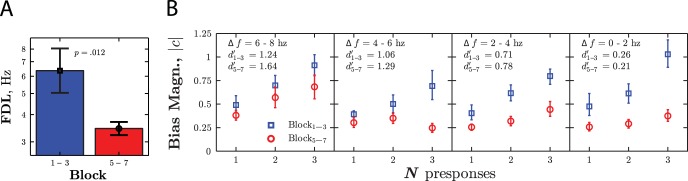
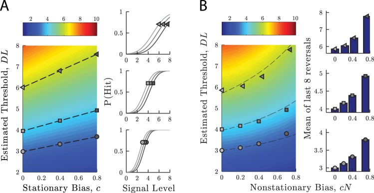
Sensory judgments improve with practice. Such perceptual learning is often thought to reflect an increase in perceptual sensitivity. However, it may also represent a decrease in response bias, with unpracticed observers acting in part on a priori hunches rather than sensory evidence. To examine whether this is the case, 55 observers practiced making a basic auditory judgment (yes/no amplitude-modulation detection or forced-choice frequency/amplitude discrimination) over multiple days. With all tasks, bias was present initially, but decreased with practice. Notably, this was the case even on supposedly "bias-free," 2-alternative forced-choice, tasks. In those tasks, observers did not favor the same response throughout (stationary bias), but did favor whichever response had been correct on previous trials (nonstationary bias). Means of correcting for bias are described. When applied, these showed that at least 13% of perceptual learning on a forced-choice task was due to reduction in bias. In other situations, changes in bias were shown to obscure the true extent of learning, with changes in estimated sensitivity increasing once bias was corrected for. The possible causes of bias and the implications for our understanding of perceptual learning are discussed.

Figure 1

A simple signal detection theory model of decision making (Green & Swets, 1974), adapted from Amitay, Zhang, Jones, and Moore, 2014. (A) The incoming physical stimulus is transformed into an internal representation by summing over n information channels, each subject to additive internal noise (the final decision variable may then be further corrupted by late sources of internal noise, not shown here for simplicity). (B) A decision is made by comparing the resultant decision variable to a criterion, λ, which may or may not be optimally placed. Sensitivity is limited by the amount of internal noise, and the observer’s ability to attend selectivity to the task-relevant information channels. Bias is limited by the placement of λ, which may be affected by a range of factors, such as the perceived likelihood of a certain response, or the perceived utility of a certain outcome (see General Discussion). This model is similar to those used in a wide range of papers, both within the perceptual learning literature (e.g., Liu, Dosher, & Lu, 2014; Jones, Moore, Shub, & Amitay, 2014), and more generally (Richards & Zhu, 1994; Tyler & Chen, 2000). Mathematically, this model could be formulated as: respond “yes” if $\left[{\displaystyle \sum _{i=1}^n{\omega }_i\left(S_i+N_i\right)}\right]$ > λ, otherwise respond “no” (where S_i is the output of the ith information channel, and N_i is a corresponding noise sample).

Figure 2

Bias is the distance between the observer’s criterion location, λ_obs (red [dark gray] dashed), and the ideal criterion location, λ_ideal (black solid). When noise (N) and signal (S) distributions have equal variance (and are sampled from with equal frequency), λ_ideal is located halfway between their means, as shown here. Here, the observer is overly liberal (biased toward indicating that a signal was present). Performance is also limited by the observer’s sensitivity (or signal-to-noise ratio), which is inversely proportional to the common area under the two distributions (highlighted in red [dark gray]). (N.B. the decision dimension is unspecified, but is typically proportional to some physical aspect of the stimulus, such as its intensity.) See the online article for the color version of this figure.

Figure 3

Experiment I: (A) Example stimuli. Showing a range of modulation depths, from zero (top) to full (bottom) modulation. (B) Learning. Group-mean ± 1 SE (bottom) detection limens as a function of session, and individual values (top) for first/last session. Individual improvements/decrements in threshold are shown by solid-green [light gray] and dashed-red [dark gray] lines, respectively. (C) Changes in global bias. Group-mean ± 1 SE (bottom) global bias (cf. Equation 2) as a function of session, and individual values (top) for first/last session. Individual improvements/decrements in bias magnitude are shown by solid-green [light gray] and dashed-red [dark gray] lines, respectively. See the online article for the color version of this figure.

Figure 4

Experiment II: Group mean (±1 SE) bias as a function of N identical presponses. The left column shows data for identical, correct presponses. The right column shows data for identical, incorrect presponses. The upper row shows signed c values (Equation 3) for Interval 1 (solid, circles) and Interval 2 (dashed, triangles) presponses. The lower row shows absolute bias magnitude, |c|, averaged across presponse identities. The numbers in parentheses give the mean number of observations (averaged over intervals and observers). The gray marker (far left) shows bias as estimated using all trials, as per classic SDT. Curves represent least-square 2nd-degree polynomial fits. See the online article for the color version of this figure.

Figure 5

Experiment III: Group mean ± 1 SE (A) Sensitivity and (B) Bias magnitude, before (blue [black], squares) and after (red [dark gray], circles) practice. Sensitivity was indexed by the 70.7% frequency discrimination limen. Bias magnitude was measured in the same way as in Figure 4, and was measured independently depending on the N presponses (abscissa) and the frequency difference between standard and comparison (panels). See the online article for the color version of this figure.

Figure 6

Simulations: Changes in estimated threshold given varying levels of: (A) stationary bias, (B) nonstationary bias. True threshold is indicated by heatmap color. Markers show estimated thresholds at three levels of bias, given a low (circle), medium (square) or high (triangles) true threshold. Dashed lines show the predicted change in estimated threshold, using the correction factors given in Equation 5 (A) or Equation 6 (B). See the online article for the color version of this figure.

References

-
- Ahissar M., & Hochstein S. (1997). Task difficulty and the specificity of perceptual learning. Nature, 387(6631), 401–406. - PubMed
- Alho K., Teder W., Lavikainen J., & Näätänen R. (1994). Strongly focused attention and auditory event-related potentials. Biological Psychology, 38, 73–90. - PubMed
- Amitay S., Hawkey D. J. C., & Moore D. R. (2005). Auditory frequency discrimination learning is affected by stimulus variability. Attention, Perception, & Psychophysics, 67, 691–698. - PubMed
Publication types
MeSH terms
Grants and funding
LinkOut - more resources
Full Text Sources
Other Literature Sources