

A computational atlas of the hippocampal formation using ex vivo, ultra-high resolution MRI: Application to adaptive segmentation of in vivo MRI
- PMID: 25936807
- PMCID: PMC4461537
- DOI: 10.1016/j.neuroimage.2015.04.042
A computational atlas of the hippocampal formation using ex vivo, ultra-high resolution MRI: Application to adaptive segmentation of in vivo MRI
Abstract
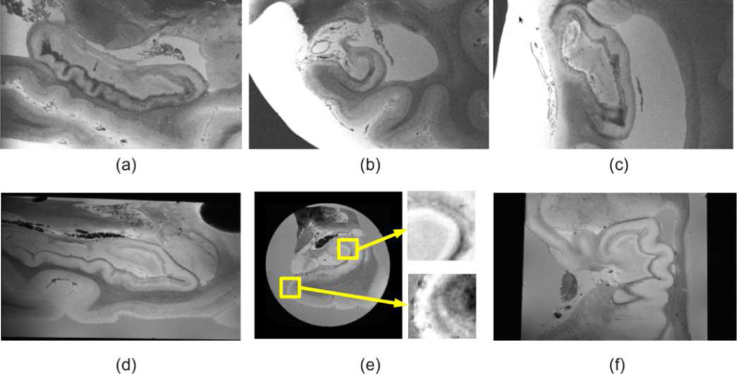
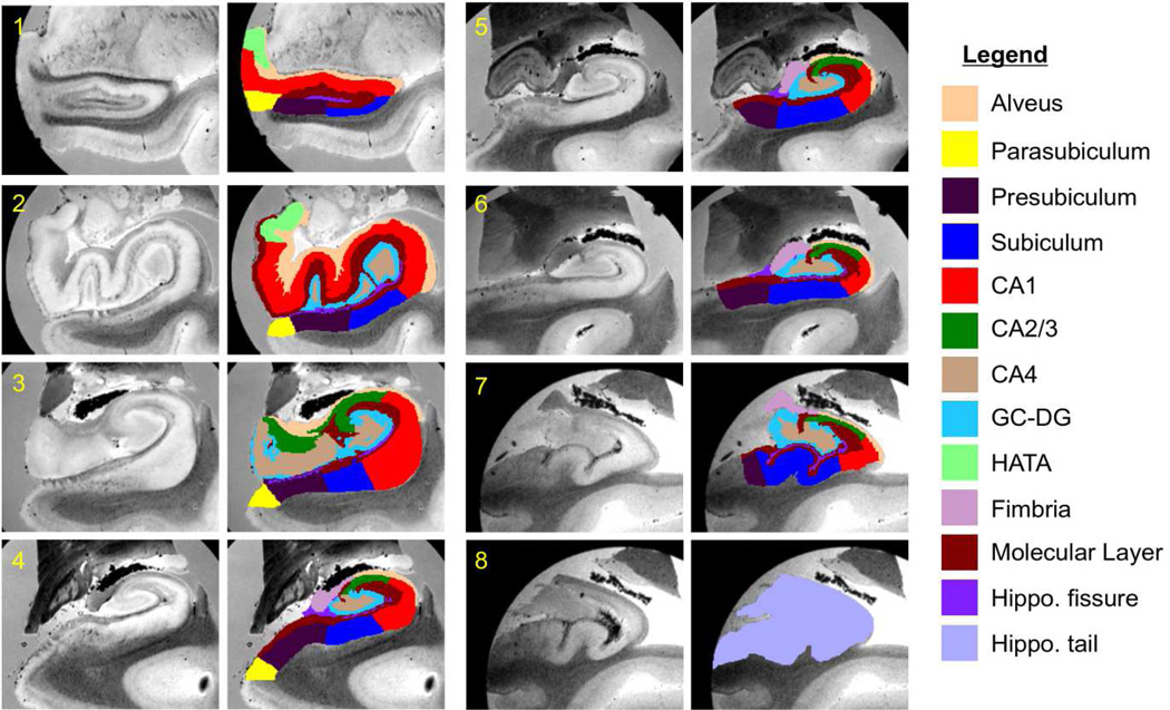
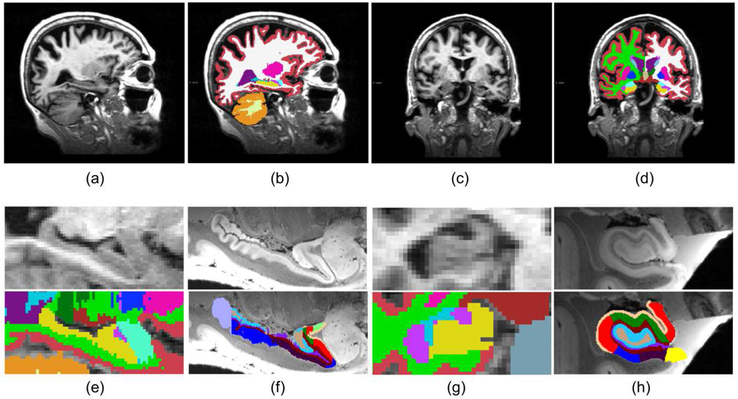
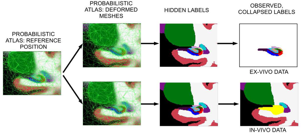
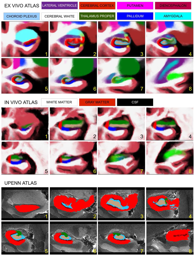
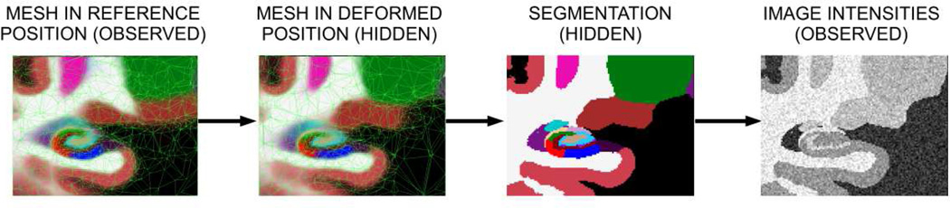
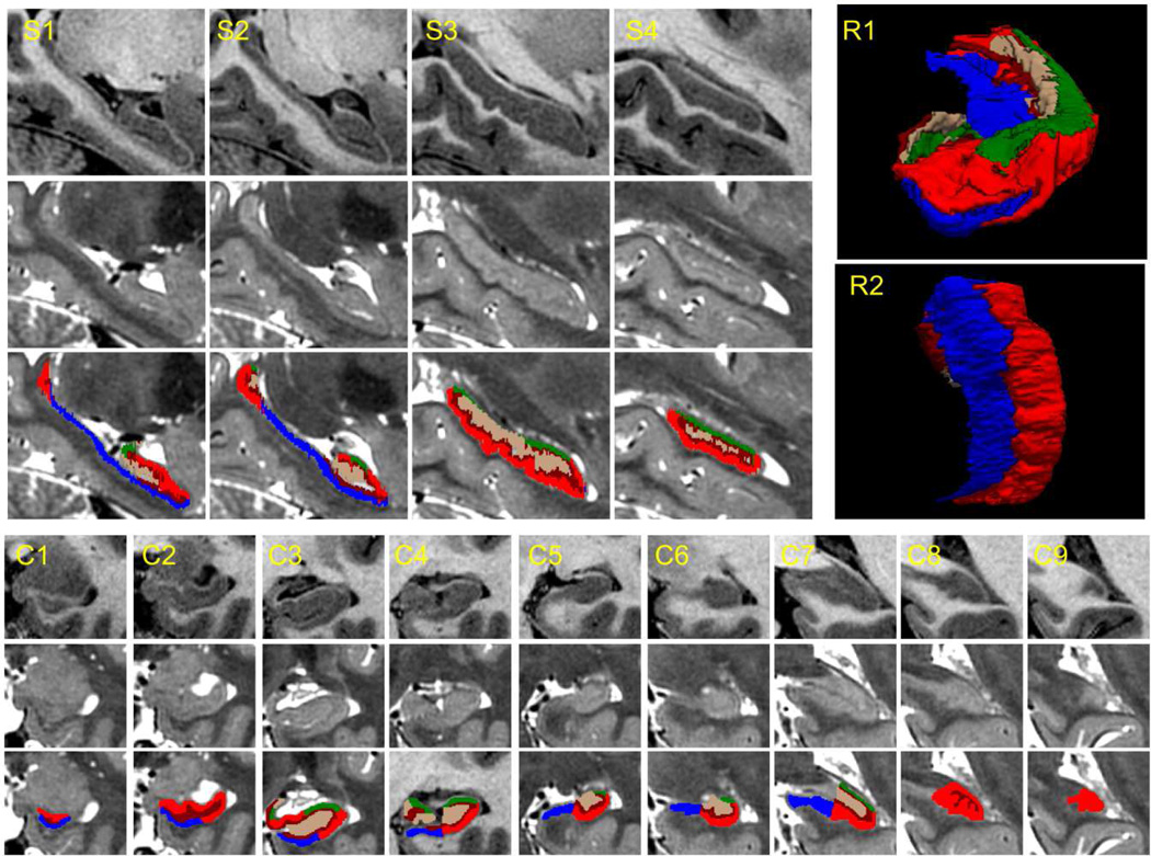
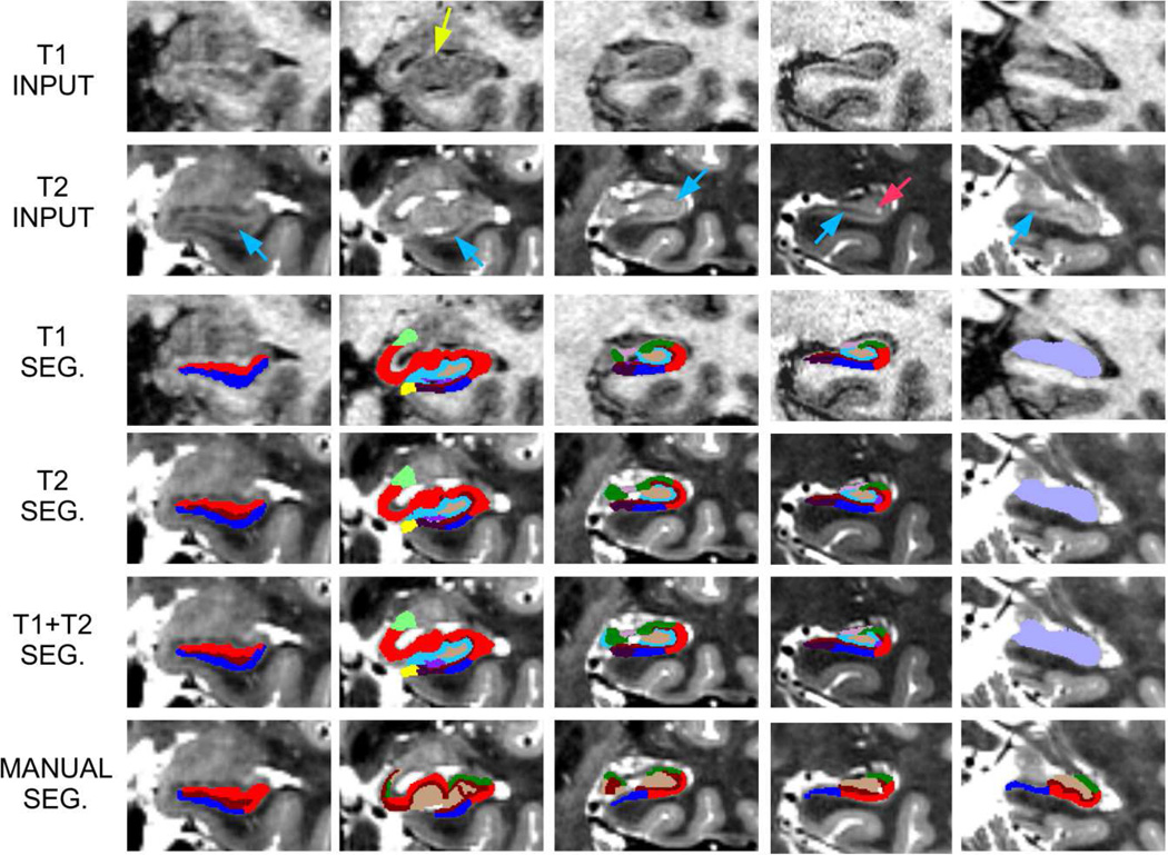
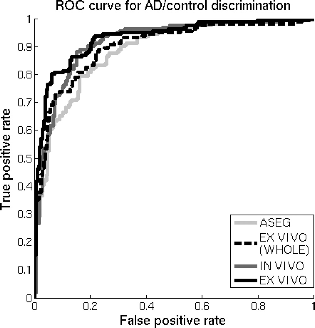
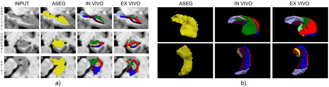
Automated analysis of MRI data of the subregions of the hippocampus requires computational atlases built at a higher resolution than those that are typically used in current neuroimaging studies. Here we describe the construction of a statistical atlas of the hippocampal formation at the subregion level using ultra-high resolution, ex vivo MRI. Fifteen autopsy samples were scanned at 0.13 mm isotropic resolution (on average) using customized hardware. The images were manually segmented into 13 different hippocampal substructures using a protocol specifically designed for this study; precise delineations were made possible by the extraordinary resolution of the scans. In addition to the subregions, manual annotations for neighboring structures (e.g., amygdala, cortex) were obtained from a separate dataset of in vivo, T1-weighted MRI scans of the whole brain (1mm resolution). The manual labels from the in vivo and ex vivo data were combined into a single computational atlas of the hippocampal formation with a novel atlas building algorithm based on Bayesian inference. The resulting atlas can be used to automatically segment the hippocampal subregions in structural MRI images, using an algorithm that can analyze multimodal data and adapt to variations in MRI contrast due to differences in acquisition hardware or pulse sequences. The applicability of the atlas, which we are releasing as part of FreeSurfer (version 6.0), is demonstrated with experiments on three different publicly available datasets with different types of MRI contrast. The results show that the atlas and companion segmentation method: 1) can segment T1 and T2 images, as well as their combination, 2) replicate findings on mild cognitive impairment based on high-resolution T2 data, and 3) can discriminate between Alzheimer's disease subjects and elderly controls with 88% accuracy in standard resolution (1mm) T1 data, significantly outperforming the atlas in FreeSurfer version 5.3 (86% accuracy) and classification based on whole hippocampal volume (82% accuracy).
Copyright © 2015. Published by Elsevier Inc.
Figures
References
-
- Acsády L, Káli S. Models, structure, function: the transformation of cortical signals in the dentate gyrus. Progress in Brain Research. 2007;163:577–599. - PubMed
-
- Apostolova L, Dinov I, Dutton R, Hayashi K, Toga A, Cummings J, et al. 3D comparison of hippocampal atrophy in amnestic mild cognitive impairment and Alzheimer's disease. Brain. 2006;129(11):2867–2873. - PubMed
-
- Arnold S, Hyman B, Flory J, Damasio A, Van Hoesen G. The topographical and neuroanatomical distribution of neurofibrillary tangles and neuritic plaques in the cerebral cortex of patients with Alzheimer's disease. Cerebral Cortex. 1991;1(1):103–116. - PubMed
Publication types
MeSH terms
Grants and funding
- P30-AG010129/AG/NIA NIH HHS/United States
- R01 NS052585-01/NS/NINDS NIH HHS/United States
- S10 RR019307/RR/NCRR NIH HHS/United States
- P30 AG013846/AG/NIA NIH HHS/United States
- R01 NS052585/NS/NINDS NIH HHS/United States
- R01EB013565/EB/NIBIB NIH HHS/United States
- P30AG13846/AG/NIA NIH HHS/United States
- P30 AG010129/AG/NIA NIH HHS/United States
- S10 RR023043/RR/NCRR NIH HHS/United States
- RC1 AT005728-01/AT/NCCIH NIH HHS/United States
- R01 EB006758/EB/NIBIB NIH HHS/United States
- R01 AG022381/AG/NIA NIH HHS/United States
- R01AG1649/AG/NIA NIH HHS/United States
- K01 AG030514/AG/NIA NIH HHS/United States
- U24 RR021382/RR/NCRR NIH HHS/United States
- U01 MH093765/MH/NIMH NIH HHS/United States
- R01 NS070963/NS/NINDS NIH HHS/United States
- R01EB006758/EB/NIBIB NIH HHS/United States
- R01 AG016495/AG/NIA NIH HHS/United States
- P30 AG062421/AG/NIA NIH HHS/United States
- R01NS083534/NS/NINDS NIH HHS/United States
- U01 AG024904/AG/NIA NIH HHS/United States
- K01-AG030514/AG/NIA NIH HHS/United States
- AG022381/AG/NIA NIH HHS/United States
- R01 AG008122/AG/NIA NIH HHS/United States
- P50 AG005134/AG/NIA NIH HHS/United States
- 1S10RR019307/RR/NCRR NIH HHS/United States
- 1S10RR023043/RR/NCRR NIH HHS/United States
- 5R01AG008122-22/AG/NIA NIH HHS/United States
- P41EB015896/EB/NIBIB NIH HHS/United States
- 1R21NS072652-01/NS/NINDS NIH HHS/United States
- RC1 AT005728/AT/NCCIH NIH HHS/United States
- 1R01NS070963/NS/NINDS NIH HHS/United States
- 1S10RR023401/RR/NCRR NIH HHS/United States
- K01 AG028521/AG/NIA NIH HHS/United States
- R01 EB013565/EB/NIBIB NIH HHS/United States
- 5U01-MH093765/MH/NIMH NIH HHS/United States
- R21 NS072652/NS/NINDS NIH HHS/United States
- P41 EB015896/EB/NIBIB NIH HHS/United States
- R01 NS083534/NS/NINDS NIH HHS/United States
- S10 RR023401/RR/NCRR NIH HHS/United States
- K01AG028521/AG/NIA NIH HHS/United States
LinkOut - more resources
Full Text Sources
Other Literature Sources
Medical
