The solvent component of macromolecular crystals

Abstract

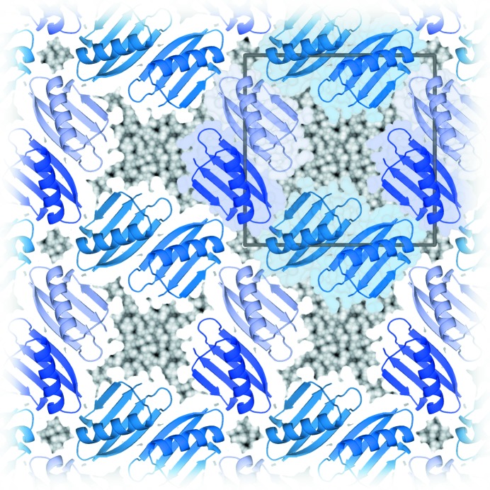
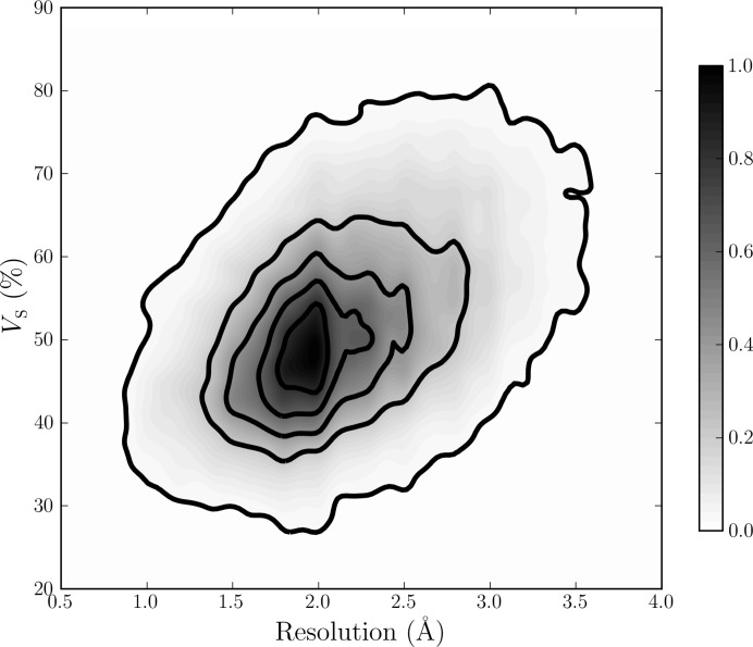
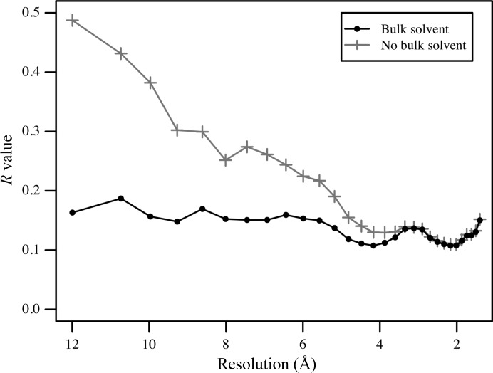
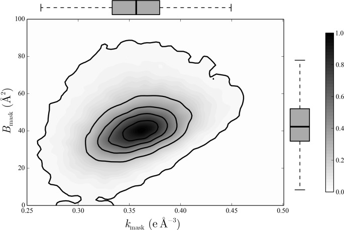
The mother liquor from which a biomolecular crystal is grown will contain water, buffer molecules, native ligands and cofactors, crystallization precipitants and additives, various metal ions, and often small-molecule ligands or inhibitors. On average, about half the volume of a biomolecular crystal consists of this mother liquor, whose components form the disordered bulk solvent. Its scattering contributions can be exploited in initial phasing and must be included in crystal structure refinement as a bulk-solvent model. Concomitantly, distinct electron density originating from ordered solvent components must be correctly identified and represented as part of the atomic crystal structure model. Herein, are reviewed (i) probabilistic bulk-solvent content estimates, (ii) the use of bulk-solvent density modification in phase improvement, (iii) bulk-solvent models and refinement of bulk-solvent contributions and (iv) modelling and validation of ordered solvent constituents. A brief summary is provided of current tools for bulk-solvent analysis and refinement, as well as of modelling, refinement and analysis of ordered solvent components, including small-molecule ligands.

Keywords: bulk solvent; macromolecular crystals; ordered solvent; solvent content.

Figure 1

Macromolecular crystals. Given favourable kinetics, macromolecules can self-assemble from a metastable, supersaturated solution into crystals, a periodic network of macromolecules connected by weak but specific intermolecular interactions. The solvent content V _S of this simple P ₄ crystal structure, PDB entry 2on8 (Wunderlich et al., 2007 ▶), is about 50%. The intermolecular regions are filled with dynamically moving solvent molecules, modelled as homogeneous bulk solvent §2.4. Its contributions to diffracted intensities are averaged over the entire molecule and over the time frame of a conventional diffraction experiment, with the dynamics of the solvent reflected in diffuse, non-Bragg scattering contributions. The region between the macro­molecules and bulk solvent may contain distinct solvent density which can be properly modelled as a part of the crystal structure. The complex and dynamic transition region from the ordered molecules to the bulk solvent is not separately modelled at present. This figure is in essence a modernised version of Figs. 1 in Bragg & Perutz (1952 ▶) and Moews & Kretsinger (1975 ▶).

Figure 2

Two-dimensional density function of V _S for 60 218 protein crystal forms using binned two-dimensional kernel estimates. The scale of V _S from 20 to 90% on the y axis corresponds to V _M values between 1.54 and 12.3 ų Da⁻¹. The plot has been normalized to have a maximum value of 1. Isocontour lines are drawn as solid bold lines in increments of 0.2. There is a clear trend towards lower values of V _S at higher resolutions. Most density is centred about approximately 1.9 Å resolution and V _S = 50%, and typical values for V _S range between 30 and 80%. Figure from Weichenberger & Rupp (2014 ▶). Owing to a 60-fold lower number of available DNA/RNA crystal structures in the PDB, the dependence of experimental resolution on solvent content cannot be established for nucleic acid chains (see Supporting Information).

Figure 3

Example of the bulk-solvent contribution to the R value shown by resolution for PDB entry 3fo3 (Trofimov et al., 2010 ▶). Solid black and grey curves show the effect of including (lower R values) versus not including (higher R values) the bulk-solvent contribution to the total model structure factors.

Figure 4

Bulk-solvent parameters. Two-dimensional density function of the bulk-solvent parameters k _mask/B _mask derived from 70 481 entries deposited in the PDB for which refinement data could reliably be extracted. Values for the mean solvent density k _mask and smearing factor B _mask were computed with PHENIX (Adams et al., 2010 ▶). The plot is limited to PDB entries with R _work between 0.05 and 0.30, only positive values for k _mask, measurements of B _mask of less than 300 and a solvent content of at least 5%. The density function was constructed using a two-dimensional kernel density estimation with an axis-aligned bivariate normal kernel and has been normalized to a maximum value of 1. Isocontour lines are plotted as solid lines at regularly spaced intervals of size 0.2. Box plots show the extents of the k _mask and B _mask distributions; the median is indicated by a thick line in the grey box, which represents the interval from the lower to the upper quartile, and whiskers extend to data points not more extreme than 1.5 times the interquartile range. The sample median of k _mask equals 0.36 (0.04) e Å⁻³ and for B _mask the sample median is 42.4 Ų. The distribution of B _mask has a small tail towards higher values, which is expressed by its sample skewness of 3.2, whereas the k _mask distribution appears to be much more symmetric about its mean, with a sample skewness of 0.43. This plot does not show 2.7% of B _mask entries and 1.7% of k _mask data, which are located outside of the limits of the axes. This figure was generated with matplotlib (Hunter, 2007 ▶).

Figure 5

Extended hydrogen-bonded water networks. (a) presents a well defined hydrogen-bond network found in PDB entry 2j9n (Viola et al., 2007 ▶). The blue mesh represents the contours of σ_A-derived maximum-likelihood 2mF _o − DF _c maps at the 1σ level, and the green arrows in the chemical scheme shown in (b) point towards the hydrogen-accepting electron lone pairs. Note that each bond has a proper donor–acceptor pair (which clearly defines the proper orientation of the Gln30 residue) and the different types of interactions: direct backbone–side chain, side chain–side chain and water-mediated interactions between residues. Typical X—O—H angles are 120° for the sp ²-hybridized orbitals of the –OH groups and 104.5° for H—O—H in the nearly tetrahedrally coordinated water O atom. The covalent O—H distance is 0.96 Å. (c) depicts a well defined water network in the intermolecular space of a high-resolution (1.2 Å) structure revealing typical, ice-like five-membered and six-membered water-ring networks, while the central water atom possesses an almost perfect tetrahedral arrangement of hydrogen-bond partners (PDB entry 1bpi; Parkin et al., 1996; figure adapted from Rupp, 2009 ▶).

Figure 6

Resolution-dependent mean number of water molecules per amino acid. The mean number of water molecules per residue is computed as the number of water molecules divided by the number of amino acids of all chains present in the asymmetric unit. This number was computed for each of the 77 346 protein structures determined by X-ray crystallo­graphy downloaded from the PDB on 23 May 2014. The figure utilizes box plots to visualize the distribution of the number of water molecules per residue observed in 0.1 Å bins in the experimental resolution range 0.6–3.5 Å. In the box plot, the grey boxes display values that fall in between the first and third quartile, the black bar represents the median and the whiskers extend to data points no more than 1.5 times the inner quartile range; data points outside this region are highlighted as black dots. The graph reflects the plausible trend that more discrete waters can be built in structures with higher resolution than in those with lower resolution. In the low-resolution range the distributions are skewed towards zero water molecules per residue, as can be read from the location of the median in these distributions. This trend holds until resolutions as low as 2.5 Å, from where on the distributions start to become symmetric. Notice that the bins for very high (better than 0.8 Å) and very low (worse than 3.3 Å) resolution are populated with fewer than 100 measurements. A corresponding plot for nucleic acid structure models displaying similar but limited information owing to the much smaller number of DNA/RNA structures determined by X-ray crystallo­graphy is provided in Supplementary Fig. S2.

Figure 7

Example of alternate conformations correlated with partial water occupancy. The Glu side chain split at C^β assumes two approximately 60/40% occupied alternate conformations. The two water atoms are too close to be present at the same time, and their occupancies should be related to those of the associated side chains. The sum of the occupancies of the two groups must be constrained to 1.0. 2mF _o − DF _c electron density is contoured at the 1σ level. This figure was modified from Rupp (2009 ▶).

Figure 8

Identification of elemental ions. (a) The central atom has electron density comparable to water but displays the typical octahedral coordination of a metal ion. The coordination distances of 2.0–2.2 Å are compatible with Mg²⁺ ions isoelectronic with the surrounding waters. PDB entry 1gkb (Kantardjieff et al., 2002 ▶). (b) An originally modelled water atom with improbably low B factors can be identified as Cl⁻ by electron-density peak height, coordination distances (3.1–3.7 Å) and its preference to bind to backbone N atoms and positively charged residues. PDB entry 1c8u (Li et al., 2000 ▶). 2mF _o − DF _c electron density is contoured at the 1σ level (blue) and the 5σ level (red). The figures are modified from Rupp (2009 ▶).

Figure 9

Fraction of occupied receptor sites plotted against ligand equilibrium concentration for three different binding constants. While in the millimolar and lower K _d range small concentrations of ligand suffice to achieve reasonable binding-site occupancy (between 70 and 90%), quite impractical concentrations of ligand in the crystallization drop are required for poor binders. On the other hand, given a sufficiently high concentration, even weakly binding (and non-native) ligands can be forced into a binding site. Figure from Pozharski et al. (2013 ▶) calculated as derived in Danley (2006 ▶) and Rupp (2009 ▶).

Figure 10

Ligands placed into density of mother-liquor components. In the structure of Bacillus cereus chitinase (PDB entry 3n1a; Hsieh et al., 2010 ▶), the cyclo-(l-His-l-Pro) molecule (CHQ-1514, chain A) is placed into low-level electron density that is difficult to interpret (a) and which may be plausibly interpreted as an acetate molecule present in the crystallization cocktail at 200 mM, supported by a newly formed hydrogen bond between Asp-143 and the suggested acetate (b). In the structure of penicillin-binding protein 4 from Staphylococcus aureus (PDB entry 3hun; Navratna et al., 2010 ▶) the phenyl moiety of the ampicillin (ZZ7-501, chain B) is placed in a region of the electron density that based on difference density analysis could be better interpreted as a sulfate ion (c). The re-refined model that includes sulfate ion is shown in (d). (e) The original, obsoleted and distorted bacteriochlorophyll model at the eighth binding site in the FMO protein from Pelodictyon phaeum (PDB entry 3oeg); (f) depicts the same region of the corrected PDB entry 3vdi (Tronrud & Allen, 2012 ▶) modelled with more plausible PEG fragments and water molecules. Electron-density maps in (a), (b), (c) and (d) are 2.0 Å resolution mF _o − DF _c OMIT difference maps contoured at ±3σ (green/red) and 2mF _o − DF _c REFMAC maximum-likelihood OMIT maps contoured at 1σ (blue). The maps shown in (e) and (f) are positive difference density OMIT mF _o − DF _c maps (3σ level, blue) after BUSTER-TNT refinement following rebuilding of the structure with phenix.autobuild without any ligand included. (a), (b), (c) and (d) are modified from Pozharski et al. (2013 ▶); (e) and (f) were kindly supplied by Dale Tronrud, Department of Biochemistry and Biophysics, Oregon State University, USA.

References

1. Abrahams, J. P. & Leslie, A. G. W. (1996). Acta Cryst. D52, 30–42. - PubMed
1. Adams, P. D. et al. (2010). Acta Cryst. D66, 213–221.
1. Adams, P. D., Pannu, N. S., Read, R. J. & Brünger, A. T. (1997). Proc. Natl Acad. Sci. USA, 94, 5018–5023. - PMC - PubMed
1. Afonine, P. V. & Adams, P. D. (2012). Comput. Crystallogr. Newsl. 3, 18–21.
1. Afonine, P. V., Grosse-Kunstleve, R. W., Adams, P. D. & Urzhumtsev, A. (2013). Acta Cryst. D69, 625–634. - PMC - PubMed
Publication types