Fine Mapping Causal Variants with an Approximate Bayesian Method Using Marginal Test Statistics

Abstract

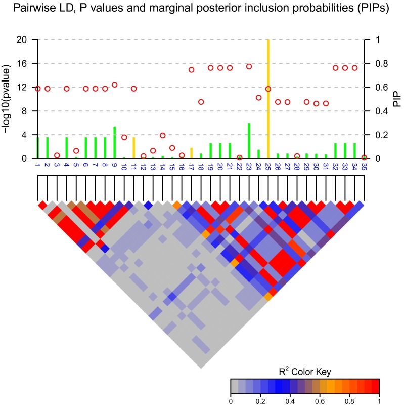
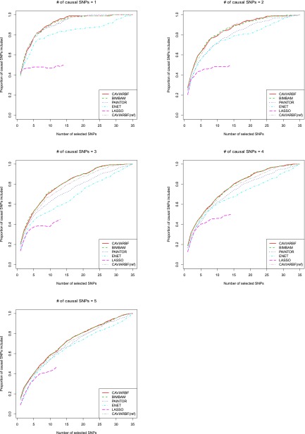
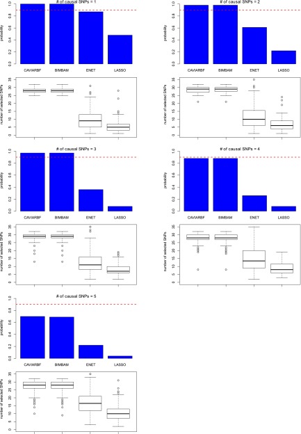
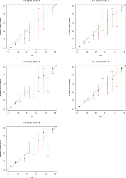
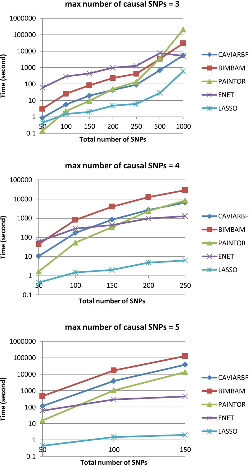
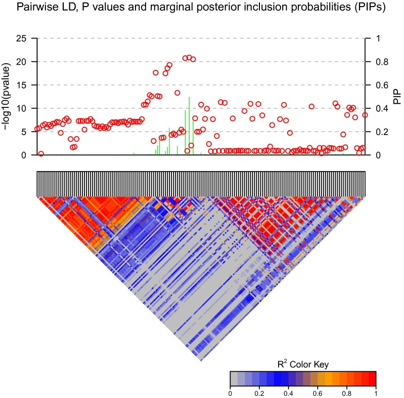
Two recently developed fine-mapping methods, CAVIAR and PAINTOR, demonstrate better performance over other fine-mapping methods. They also have the advantage of using only the marginal test statistics and the correlation among SNPs. Both methods leverage the fact that the marginal test statistics asymptotically follow a multivariate normal distribution and are likelihood based. However, their relationship with Bayesian fine mapping, such as BIMBAM, is not clear. In this study, we first show that CAVIAR and BIMBAM are actually approximately equivalent to each other. This leads to a fine-mapping method using marginal test statistics in the Bayesian framework, which we call CAVIAR Bayes factor (CAVIARBF). Another advantage of the Bayesian framework is that it can answer both association and fine-mapping questions. We also used simulations to compare CAVIARBF with other methods under different numbers of causal variants. The results showed that both CAVIARBF and BIMBAM have better performance than PAINTOR and other methods. Compared to BIMBAM, CAVIARBF has the advantage of using only marginal test statistics and takes about one-quarter to one-fifth of the running time. We applied different methods on two independent cohorts of the same phenotype. Results showed that CAVIARBF, BIMBAM, and PAINTOR selected the same top 3 SNPs; however, CAVIARBF and BIMBAM had better consistency in selecting the top 10 ranked SNPs between the two cohorts. Software is available at https://bitbucket.org/Wenan/caviarbf.

Keywords: Bayesian fine mapping; causal variants; marginal test statistics.

Figure 1

P-values and posterior inclusion probabilities (PIPs). Circles represent the individual SNP-based P-values on the left y-axis and lines represent the PIPs on the right y-axis. The gold color indicates the true causal SNPs. The color-coded LD pattern is shown below. The noncausal variant (SNP23) has the smallest P-values, but is purely due to high LD with the causal variant (SNP17) and statistical fluctuation. The causal variant (SNP25) does not achieve the smallest P-values but is correctly captured by the highest PIP.

Figure 2

Comparison of different fine-mapping methods on quantitative traits. The y-axis is the proportion of causal SNPs included and the x-axis is the number of selected SNPs. There are 35 SNPs in total. The proportions are calculated over 100 data sets. The proportion (y-value) is not calculated if >5 data sets do not reach the specified number of SNPs (x-value). This is why some proportions are not available for LASSO as the number of selected candidate SNPs becomes large. Each plot corresponds to a different number of causal SNPs.

Figure 3

Comparison of different prior values ${\sigma }_a$ on quantitative traits. CAVIARBF is used to calculate the Bayes factors. The description of the x-axis and y-axis is the same as in Figure 2.

Figure 4

Comparison of different criteria to prioritize variants on quantitative traits. CAVIARBF is used to calculate the Bayes factors. The green dashed line represents prioritizing SNPs using marginal posterior inclusion probabilities (PIPs). The red solid line represents prioritizing SNPs using the ρ-level confidence set. The description of the x-axis and y-axis is the same as in Figure 2.

Figure 5

Estimated probabilities of the ρ-level confidence set and boxplots of the number of selected SNPs. The phenotypes are quantitative traits. The bar graph is plotted above the corresponding boxplot. The red dashed line shows the nominal level of the confidence set. The bars show the estimated proportion where the selected SNPs include all causal SNPs among 100 data sets. For ENET and LASSO, the best model selected by cross-validation is used for each data set.

Figure 6

Calibration of the posterior inclusion probabilities (PIPs) on quantitative traits. CAVIARBF is used to calculate the Bayes factors. SNPs were put into 10 bins of width 0.1 according to their PIPs. In each bin, the proportion of causal SNPs was then calculated. The x-axis shows the center of each bin. The y-axis is the proportion of causal SNPs. The blue points show the proportion of causal SNPs in each bin. The red bars show the 95% Wilson score confidence interval of the proportion assuming a binomial distribution in each bin. One hundred data sets were used in each plot. Except those points with very large confidence intervals due to small total counts in the bins, usually <10, in general the points lie near the line y = x. This indicates that the PIPs are reasonably calibrated.

Figure 7

Time cost of different methods. Different maximal numbers of causal SNPs are tested for CAVIARBF, BIMBAM, and PAINTOR. The y-axis is on a log10 scale. The x-axis shows the total number of SNPs in the input data.

Figure 8

P-values and posterior inclusion probabilities (PIPs) from CAVIARBF on the U.S. cohort. Circles represent the individual SNP-based P-values on the left y-axis and lines represent the PIPs on the right y-axis. The color-coded LD pattern is shown below.

References

1. Abecasis G. R., Auton A., Brooks L. D., DePristo M. A., Durbin R. M., et al. , 2012. An integrated map of genetic variation from 1,092 human genomes. Nature 491: 56–65. - PMC - PubMed
1. Altshuler D. M., Gibbs R. A., Peltonen L., Dermitzakis E., Schaffner S. F., et al. , 2010. Integrating common and rare genetic variation in diverse human populations. Nature 467: 52–58. - PMC - PubMed
1. Armitage P., 1955. Tests for linear trends in proportions and frequencies. Biometrics 11: 375–386.
1. Durrant C., Zondervan K. T., Cardon L. R., Hunt S., Deloukas P., et al. , 2004. Linkage disequilibrium mapping via cladistic analysis of single-nucleotide polymorphism haplotypes. Am. J. Hum. Genet. 75: 35–43. - PMC - PubMed
1. ENCODE Project Consortium , 2012. An integrated encyclopedia of DNA elements in the human genome. Nature 489: 57–74. - PMC - PubMed
Publication types