Is this the right normalization? A diagnostic tool for ChIP-seq normalization

Abstract

Background: Chip-seq experiments are becoming a standard approach for genome-wide profiling protein-DNA interactions, such as detecting transcription factor binding sites, histone modification marks and RNA Polymerase II occupancy. However, when comparing a ChIP sample versus a control sample, such as Input DNA, normalization procedures have to be applied in order to remove experimental source of biases. Despite the substantial impact that the choice of the normalization method can have on the results of a ChIP-seq data analysis, their assessment is not fully explored in the literature. In particular, there are no diagnostic tools that show whether the applied normalization is indeed appropriate for the data being analyzed.

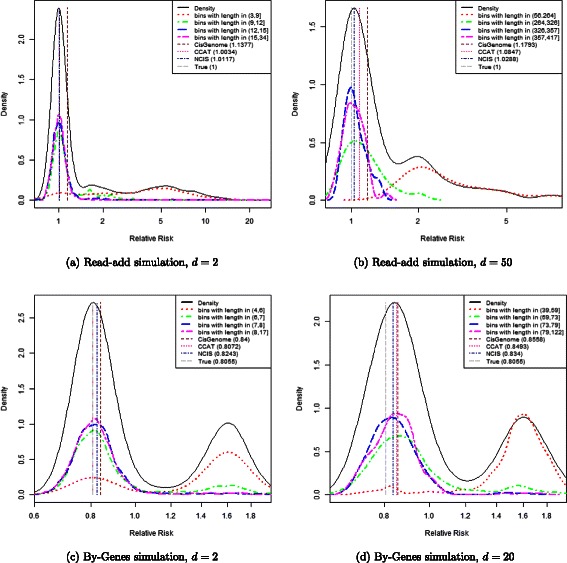
Results: In this work we propose a novel diagnostic tool to examine the appropriateness of the estimated normalization procedure. By plotting the empirical densities of log relative risks in bins of equal read count, along with the estimated normalization constant, after logarithmic transformation, the researcher is able to assess the appropriateness of the estimated normalization constant. We use the diagnostic plot to evaluate the appropriateness of the estimates obtained by CisGenome, NCIS and CCAT on several real data examples. Moreover, we show the impact that the choice of the normalization constant can have on standard tools for peak calling such as MACS or SICER. Finally, we propose a novel procedure for controlling the FDR using sample swapping. This procedure makes use of the estimated normalization constant in order to gain power over the naive choice of constant (used in MACS and SICER), which is the ratio of the total number of reads in the ChIP and Input samples.

Conclusions: Linear normalization approaches aim to estimate a scale factor, r, to adjust for different sequencing depths when comparing ChIP versus Input samples. The estimated scaling factor can easily be incorporated in many peak caller algorithms to improve the accuracy of the peak identification. The diagnostic plot proposed in this paper can be used to assess how adequate ChIP/Input normalization constants are, and thus it allows the user to choose the most adequate estimate for the analysis.

Figure 1

Diagnostic plots for mouse data. Diagnostic plots for six datasets, representing three different modifications, from the mouse embryonic fibroblast cells in the study of [38]. Panel (a) refers to H3K4me3, panel (b) to H3K27me3, panels (c-e) to the three replicates of H3K36me3, finally panel (f) to the pooled version of H3K36me3. The five densities are: the density of $log\frac{{Ñ}_{\mathit{\text{ch}}}\left(i\right)}{{Ñ}_{\mathit{\text{in}}}\left(i\right)}$ in all bins (solid black curve), the density of the subset of bins in last quartile in length (two-dashed pink), the density of the subset of bins in third quartile in length (dashed blue), the density of the subset of bins in second quartile in length (dot-dashed green), and the density of the subset of bins in first quartile in length (dotted red). The vertical lines show the estimated logr using CisGenome (brown line), CCAT (deepink line) and NCIS (navy line). The plot was produced with K=200.

Figure 2

Distributions of estimated log relative risks. The empirical density of the log relative risks for background read counts that are distributed as Poisson (solid black); or as over-dispersed Poisson with p=0.5 (dot-dashed pink) and with p=0.25 (dash blue). The solid vertical line is l o g(r), with r=0.7. The peak is around logr for all three densities.

Figure 3

Diagnostic plots for simulated data. Diagnostic plots for four simulated datasets, generated from the control sample of the ChIP-seq study by [37]. Figures (a) and (b) are the results from the Read-add simulation, with down-sampling by 2 and 50, respectively. Figures (c) and (d) are the results from the By-Genes simulation, with down-sampling by 2 and 20. The five densities are: the density of $log\frac{{Ñ}_{\mathit{\text{ch}}}\left(i\right)}{{Ñ}_{\mathit{\text{in}}}\left(i\right)}$ in all bins (solid black curve), the density of the subset of bins in last quartile in length (two-dashed pink), the density of the subset of bins in third quartile in length (dashed blue), the density of the subset of bins in second quartile in length (dot-dashed green), and the density of the subset of bins in first quartile in length (dotted red). The vertical lines show the estimated logr using CisGenome (brown line), CCAT (deepink line) and NCIS (navy line), as well as the true normalization factor in gray. The plot was produced with K=500.

Figure 4

Diagnostic plots for modENCODE data. Diagnostic plots for the three datasets from modENCODE. Datasets refer to H3K27me3 modification in D melanogaster. Panel (a) refers to ChIP id. 1820 and Input id. 1815, panel (b) to ChIP id 1957 and Input id 1961, panel (c) to the pooled version of the modEncode semples. The five densities are: the density of $log\frac{{Ñ}_{\mathit{\text{ch}}}\left(i\right)}{{Ñ}_{\mathit{\text{in}}}\left(i\right)}$ in all bins (solid black curve), the density of the subset of bins in last quartile in length (two-dashed pink), the density of the subset of bins in third quartile in length (dashed blue), the density of the subset of bins in second quartile in length (dot-dashed green), and the density of the subset of bins in first quartile in length (dotted red). The vertical lines show the estimated logr using CisGenome (brown line), CCAT (deepink line) and NCIS (navy line). The plot was produced with K=200.