QCD and strongly coupled gauge theories: challenges and perspectives

Abstract

We highlight the progress, current status, and open challenges of QCD-driven physics, in theory and in experiment. We discuss how the strong interaction is intimately connected to a broad sweep of physical problems, in settings ranging from astrophysics and cosmology to strongly coupled, complex systems in particle and condensed-matter physics, as well as to searches for physics beyond the Standard Model. We also discuss how success in describing the strong interaction impacts other fields, and, in turn, how such subjects can impact studies of the strong interaction. In the course of the work we offer a perspective on the many research streams which flow into and out of QCD, as well as a vision for future developments.

Fig. 1

Valence distribution of the pion obtained in [59] from a fit to the E615 Drell–Yan data [60] at $Q=4$ GeV, compared to the NLO parameterizations of [61] Sutton–Martin–Roberts–Stirling (SMRS) and [62] Glück–Reya–Schienbein (GRS) and to the distribution obtained from Dyson–Schwinger equations by Hecht et al. [63]. From [59]

Fig. 2

Factorization for SIDIS of extra gluons into gauge links (double lines). Figure from [66]

Fig. 3

(Upper figure) Gluon–gluon luminosity to produce a resonance of mass $M_X$ for different PDFs normalized to that of NNPDF 2.3. (Lower figure) The corresponding uncertainties in the Higgs cross section from PDFs and ${\mathit{\alpha }}_{\mathrm{s}}(M_Z)$. Figures from [136]

Fig. 4

Fit using the NLO BK nonlinear evolution equations of the combined H1/ZEUS HERA data. Figure from [161]

Fig. 5

Connections among various partonic amplitudes in QCD. The abbreviations are explained in the text

Fig. 6

The dependence of the nucleon’s isovector electric form factor $G_{\mathrm{E}}$ on the Euclidean four-momentum transfer $Q^2=-q^2$ for near-physical pion masses, as reported by the LHP Collaboration [231] and the Mainz group [232]. The phenomenological parameterization of experimental data is from [233]

Fig. 7

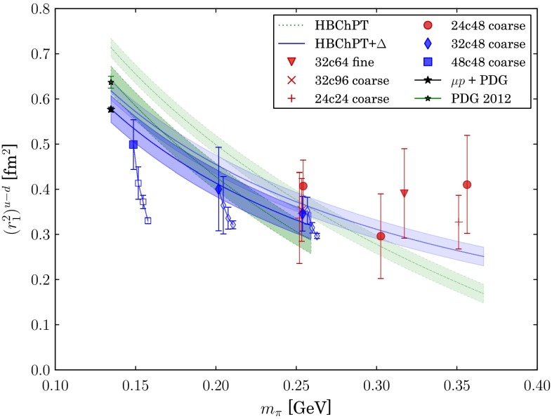
The dependence of the isovector Dirac radius $⟨r_1^2⟩$ on the pion mass from [234]. Filled blue symbols denote results based on summed operator insertions, designed to suppress excited-state contamination

Fig. 8

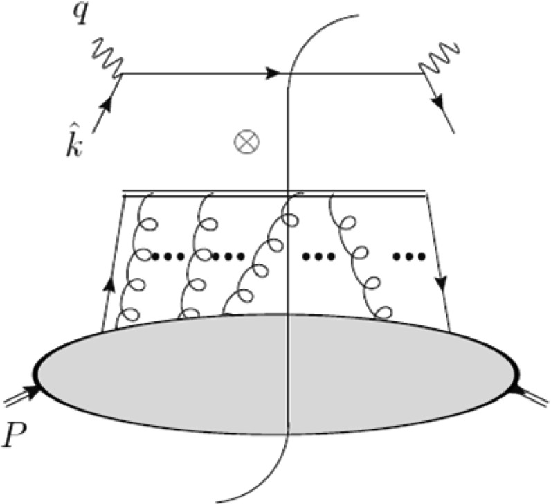
The dependence of the first moment of the isovector PDF plotted versus the pion mass. Lattice results are compiled from [, , , –253]

Fig. 9

Compilation of recent published results for the axial charge in QCD with $N_{\mathrm{f}}=2+1+1$ dynamical quarks [248] (upper panel), $N_{\mathrm{f}}=2+1$ [234, 237] (middle panel), as well as two-flavor QCD [236, 247, 255, 256] (lower panel)

Fig. 10

The vector meson, nucleon, and $\mathrm{\Delta }$/$\mathrm{\Omega }$ masses as a function of the pion mass squared in the Poincaré-covariant Faddeev approach (adapted from [278])

Fig. 11

The nucleons’ electromagnetic form factors in the Poincaré-covariant Faddeev approach (adapted from [265])

Fig. 12

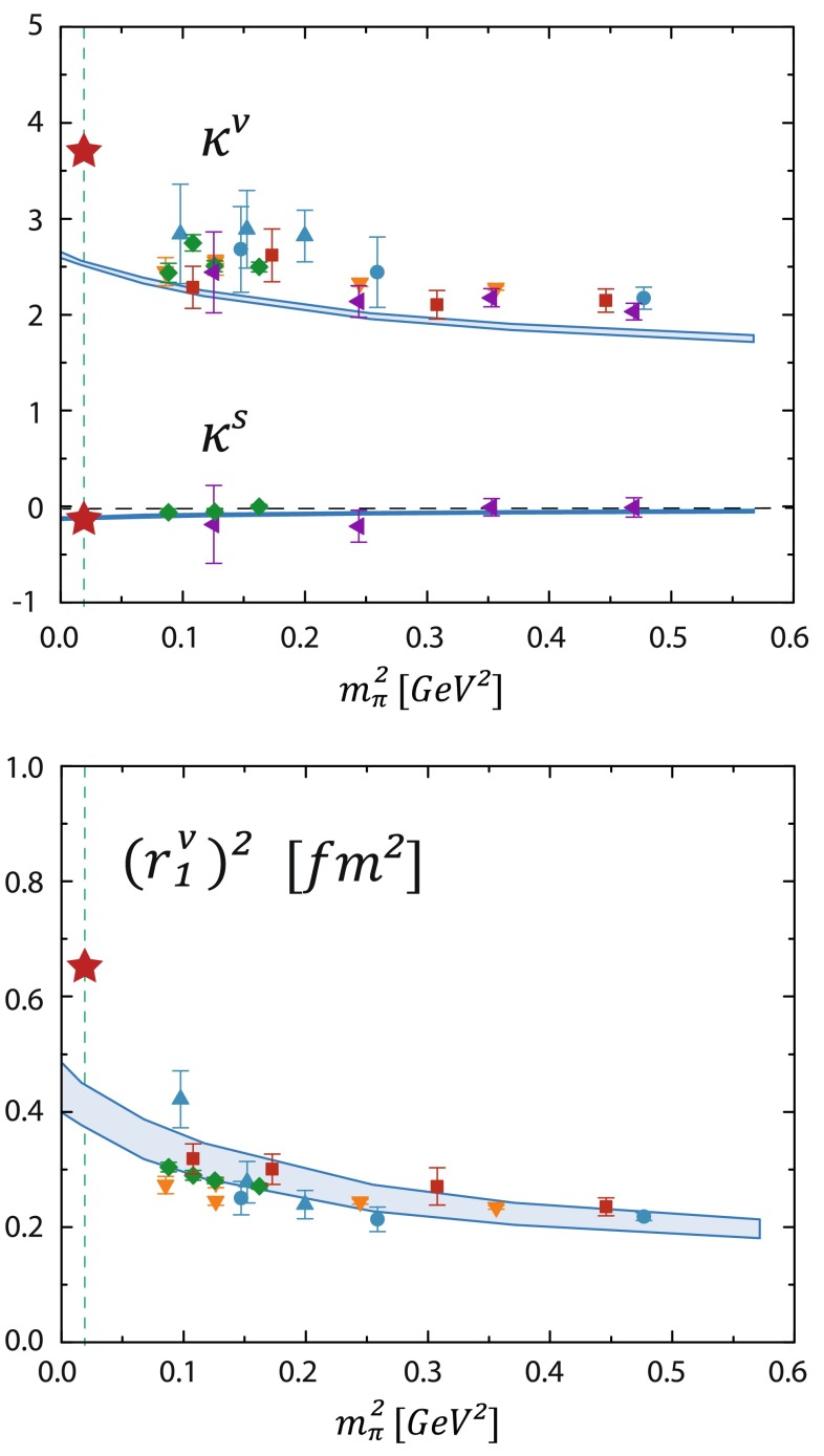
Results for the nucleon’s isoscalar and isovector anomalous magnetic moments and isovector Dirac radius in the Poincaré-covariant Faddeev approach as compared to lattice QCD results and experiment (stars) (adapted from [265])

Fig. 13

$Q^2$-evolution of the ratio of the proton’s electric form factor to a dipole form factor in the Poincaré-covariant Faddeev approach as compared to experimental data (adapted from [265])

Fig. 14

Proton radius determinations from (i) the muonic-hydrogen Lamb shift (left), (ii) electron–proton scattering (right), and (iii) the CODATA-2010 combination of the latter with ordinary hydrogen spectroscopy (center). Data taken from [290]

Fig. 15

Determination of the pion polarizability at COMPASS through the process ${\mathit{\pi }}^{-}\mathrm{Ni}\to {\mathit{\pi }}^{-}\mathit{\gamma }\mathrm{Ni}$ [337]

Fig. 16

Hadron spectrum from lattice QCD. Wide-ranging results are from MILC [361, 362], PACS-CS [349], BMW [350], and QCDSF [363]. Results for $\mathit{\eta }$ and ${\mathit{\eta }}^{\prime }$ are from RBC & UKQCD [364], Hadron Spectrum [365] (also the only $\mathit{\omega }$ mass), and UKQCD [366]. Symbol shape denotes the formulation used for sea quarks. Asterisks represent anisotropic lattices. Open symbols denote the masses used to fix parameters. Filled symbols (and asterisks) denote results. Red, orange, yellow, green, and blue stand for increasing numbers of ensembles (i.e., lattice spacing and sea quark mass). Horizontal bars (gray boxes) denote experimentally measured masses (widths). Adapted from [360]

Fig. 17

Light-quark meson spectrum resulting from lattice QCD [365], sorted by the quantum numbers $J^{\mathrm{PC}}$. Note that these results have been obtained with an unphysical pion mass, $m_{\mathit{\pi }}=396\mathrm{MeV}$

Fig. 18

Glueball masses resulting from unquenched lattice QCD [388], compared with experimental meson masses [1, 389]. From [388]

Fig. 19

Invariant mass of ${\mathit{\pi }}^{+}{\mathit{\pi }}^{-}$ and ${\mathit{\pi }}^0{\mathit{\pi }}^0$ with the ${\mathit{\pi }}^{+}{\mathit{\pi }}^{-}{\mathit{\pi }}^0$ ($3{\mathit{\pi }}^0$) mass in the $\mathit{\eta }(1405)$ mass region, measured at BES III [453]

Fig. 20

Invariant mass distribution of $\mathit{\eta }\mathit{\eta }$ from $J/\mathit{\psi }\to \mathit{\gamma }\mathit{\eta }\mathit{\eta }$, and the projection of the PWA fit from BES III [456]

Fig. 21

Exotic $1^{-+}{1}^{+}\mathit{\rho }\mathit{\pi }P$ wave observed at the COMPASS experiment [467] for 4-momentum transfer between $0.1$ and $1.0{\mathrm{GeV}}^2$ on a Pb target and ${\mathit{\pi }}^{-}{\mathit{\pi }}^{-}{\mathit{\pi }}^{+}$ final state. Left intensity, right phase difference from the $1^{++}{0}^{+}\mathit{\rho }\mathit{\pi }S$ wave as a function of the $3\mathit{\pi }$ invariant mass. The data points represent the result of the fit in mass bins, the lines are the result of the mass-dependent fit

Fig. 22

Comparison of waves for $\mathit{\eta }\mathit{\pi }$ (red data points) and ${\mathit{\eta }}^{\prime }\mathit{\pi }$ (black data points) final states. Top Intensity of the $J^{\mathrm{PC}}=2^{++}$ $D$ wave, bottom intensity of the spin-exotic $1^{-+}$ $P$ wave from COMPASS [494]

Fig. 23

Invariant mass projections from the analyses of a, b ${\mathit{\chi }}_{c1}\to \mathit{\eta }{\mathit{\pi }}^{+}{\mathit{\pi }}^{-}$, and c, d ${\mathit{\chi }}_{c1}\to {\mathit{\eta }}^{\prime }{\mathit{\pi }}^{+}{\mathit{\pi }}^{-}$ measured by CLEO-c [496]. The contributions of the individual fitted decay modes are indicated by lines, the data points with full points

Fig. 24

Intensity of the $1^{-+}{1}^{\pm }\mathit{\rho }\mathit{\pi }P$ waves from photoproduction at (left) CLAS [499] and (right) COMPASS [488] as a function of $3\mathit{\pi }$ invariant mass

Fig. 25

Double-polarization observable $G$ measured at CBELSA [515], (left) as a function of $cos{\mathit{\theta }}_{\mathit{\pi }}$ for four different photon energies, (right) as a function of photon energy for two different pion polar angles ${\mathit{\theta }}_{\mathit{\pi }}$, compared to predictions by different PWA formalisms, (blue) SAID, (red) BnGa, (black) MAID

Fig. 26

Beam-recoil observable $C_z$ for circularly polarized photons in the reaction $\mathit{\gamma }p\to K^{+}\mathrm{\Lambda }$ as a function of $\mathit{\gamma }$–$p$ CM energy for different kaon polar angles ${\mathit{\theta }}_K^{\mathrm{CM}}$ measured by CLAS [516]. The data points are compared to different models (see [516] for details)

Fig. 27

Compilation of recently published lattice QCD results for the leading hadronic vacuum polarization contribution to the muon’s anomalous magnetic moment. Displayed is ${10}^{10}{a}_{\mathit{\mu }}^{\mathrm{VP};\mathrm{had}}$, from ETM [672, 676], CLS/Mainz [674], RBC/UKQCD [673] and Aubin et al. [671]. The position and width of the red vertical line denote the phenomenological result from dispersion theory and its uncertainty, respectively

Fig. 28

The scale dependence of the electroweak mixing angle in the $\overline{}\}MS$ scheme. The blue band is the theoretical prediction, while its width denotes the theoretical uncertainty from strong interaction effects. From [1]

Fig. 29

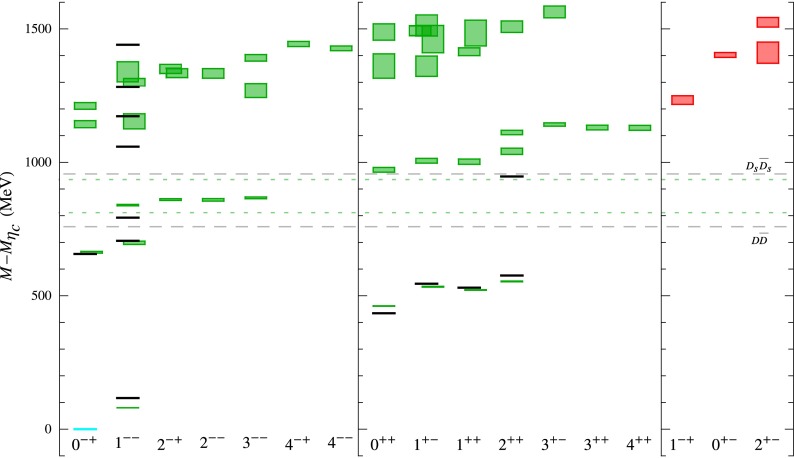
The charmonium spectrum from lattice simulations of the Hadron Spectrum Collaboration using $N_{\mathrm{f}}=2+1$ flavors of dynamical light quarks and a relativistic valence charm quark on anisotropic lattices. The shaded boxes indicate the $1\mathit{\sigma }$ confidence interval from the lattice for the masses relative to the simulated ${\mathit{\eta }}_{\mathrm{c}}$ mass, while the corresponding experimental mass differences are shown as black lines. The $D\overline{D}$ and $D_{\mathrm{s}}{\overline{D}}_{\mathrm{s}}$ thresholds from lattice simulation and experiment are shown as green and grey dashed lines, respectively. From [812]

Fig. 30

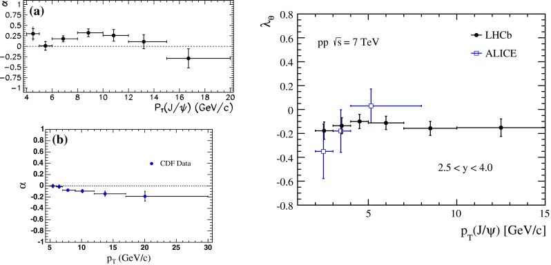
The $J/\mathit{\psi }$ polarization parameter $\mathit{\alpha }\equiv {\mathit{\lambda }}_{\mathit{\theta }}$ in the helicity frame as measured by CDF in Tevatron run I [1158] (a), run II [1159] (b), and by ALICE [1160] and LHCb [1161] at the LHC (right). Adapted from [1158, 1159, 1161], respectively

Fig. 31

The polarization parameter ${\mathit{\lambda }}_{\mathit{\theta }}$ in the helicity frame for $J/\mathit{\psi }$ (left) and $\mathit{\psi }(2S)$ (right) production as measured by CMS [1162]. Adapted from [1162]

Fig. 32

The $\mathrm{{\rm Y}}(1S)$ polarization parameter ${\mathit{\lambda }}_{\mathit{\theta }}$ in the helicity frame as measured by CDF [1156, 1163], D0 [1164] and CMS [1165]. Adapted from [1163, 1165], respectively

Fig. 33

The predictions of the $J/\mathit{\psi }$ total $e^{+}{e}^{-}$ cross section measured by Belle [1174], the transverse momentum distributions in photoproduction measured by H1 at HERA [1171, 1185], and in hadroproduction measured by CDF [1141] and ATLAS [1142], and the polarization parameter ${\mathit{\lambda }}_{\mathit{\theta }}$ measured by CDF in Tevatron run II [1159]. The predictions are plotted using the values of the CO LDMEs given in [770], [1181] and [1183] and listed in Table 13. The error bars of graphs a–g refer to scale variations, of graph d also fit errors, errors of graph h according to [1181]. As for graphs i–l, the central lines are evaluated with the default set, and the error bars evaluated with the alternative sets of the CO LDMEs used in [1183] and listed in Table 13. From [1186]

Fig. 34

Direct and indirect determinations of the $W$-boson and $t$-quark masses within the SM from measurements at LEP [698] and the Tevatron [1288], and from Higgs mass $M_{\mathrm{H}}$ measurements at the LHC [1283, 1284]. The nearly elliptical contours indicate constraints from global fits to electroweak data, note http://cern.ch/gfitter [1290], exclusive of direct measurements of $M_W$ and $m_t$ from LEP and the Tevatron [1289, 1291]. The smaller (larger) contours include (exclude) the Higgs mass determinations from the LHC. We show a September, 2013 update from a similar figure in [1289] and refer to it for all details

Fig. 35

Values of $\mathit{\sigma }/{\mathit{\sigma }}_{\mathrm{SM}}$ for particular decay modes, or of subcombinations therein which target particular production mechanisms. The horizontal bars indicate $\pm 1\mathit{\sigma }$ errors including both statistical and systematic uncertainties; the vertical band shows the overall uncertainty. The quantity $\mathit{\sigma }/{\mathit{\sigma }}_{\mathrm{SM}}$ (denoted $\mathit{\mu }(x,y)$ in text) is the production cross section times the branching fraction, relative to the SM expectation [1286]. (Figure reproduced from [1286], courtesy of the CMS collaboration.)

Fig. 36

Inclusive cross section for top pair production with center-of-mass energy in $pp$ and $p\overline{p}$ collisions [1307], compared with experimental cross sections from CDF, D0, ATLAS, and CMS [1314]. (Figure reproduced from [1314], courtesy of the CMS collaboration.)

Fig. 37

Summary of the latest dynamical calculations of the neutron EDM [–1448] $d_n$ as a function of $m_{\mathit{\pi }}^2$ from a nonzero $\overline{\mathit{\theta }}$ term in QCD. The band is a global extrapolation at 68 % CL combining all the lattice points (except for [1448]) each weighted by its error bar. The leftmost star indicates the value at the physical pion mass. Figure taken from [1449]

Fig. 38

Figures adapted from [203]. (Upper figure) Global analysis of all $N_{\mathrm{f}}=2+1(+1)$ lattice calculations of $g_{\mathrm{T}}$ (upper) and $g_{\mathrm{S}}$ (lower) [206, 234, 251, 261, 1458] with $m_{\mathit{\pi }}L>4$ and $m_{\mathit{\pi }}T>7$ cuts to avoid systematics due to small spatial or temporal extent. The leftmost points are the extrapolated values at the physical pion mass. The two bands show extrapolations with different upper pion-mass cuts: $m_{\mathit{\pi }}^2<0.4$ and $m_{\mathit{\pi }}^2<0.2$. The $m_{\mathit{\pi }}L<4$ data points are marked faded within each calculation; the lattice spacings for each point are denoted by a solid line for $a\le 0.06$ fm, dashed $0.06<a\le 0.09$ fm, dot–dashed $0.09<a\le 0.12$ fm, and dotted $a>0.12$ fm. (Lower figure) The allowed ${\mathit{ϵ}}_S$–${\mathit{ϵ}}_T$ parameter region using different experimental and theoretical inputs. The outermost (green), middle (purple), and innermost (magenta) dashed lines are the constraints from the first LHC run [1463], along with near-term expectations, running to a scale of 2 GeV to compare with the low-energy experiments. The inputs for the low-energy experiments assume that limits (at 68 % CL) of $|b|<{10}^{-3}$ and $|B_{\mathrm{BSM}}-b|<{10}^{-3}$ from neutron $\mathit{\beta }$ decay and a limit of $g_{\mathrm{T}}{\mathit{ϵ}}_{\mathrm{T}}<2\times {10}^{-4}$ from ${}^6$He $\mathit{\beta }$ decay [1464], which is a purely Gamow–Teller transition. These low-energy experiments probe $S,T$ interactions through possible interference terms and yield constraints on $\mathrm{Re}({\mathit{ϵ}}_{\mathrm{T}})$ and $\mathrm{Re}({\mathit{ϵ}}_{\mathrm{S}})$ only

Fig. 39

Compilation of $g_A$ determined from experiment (top) and lattice QCD (bottom) adapted from Ref. [1437]. The lower panel shows $g_A$ values after extrapolating to the physical pion mass collected from dynamical 2+1-flavor and 2-flavor lattice calculations using $O(a)$-improved fermions [, , , , , –, , , –, , –1472]. A small discrepancy persists: while calculations continue to tend towards values around 1.22 with a sizeable error, the experimental values are converging towards $1.275\pm 0.005$. A significant lattice effort will be necessary to reduce the systematics and achieve total error at the percent level

Fig. 40

Constraints on the (neutral-current) weak couplings of the $u$ and $d$ quarks plotted in the $C_{1u}$–$C_{1d}$ plane. The band refers to the limits from APV, whereas the more vertical ellipse represents a global fit to the existing PVES data with $Q^2<0.63{(\mathrm{GeV})}^2$. The small, more horizontal ellipse refers to the constraint determined from combining the APV and PVES data. The SM prediction as a function of ${sin}^2{\mathit{\theta }}_W$ in the $\overline{\mathrm{MS}}$ scheme appears as a diagonal line; the SM best fit value is ${sin}^2{\mathit{\theta }}_W=0.23116$ [1]. Figure taken from [1321], and we refer to it for all details

Fig. 41

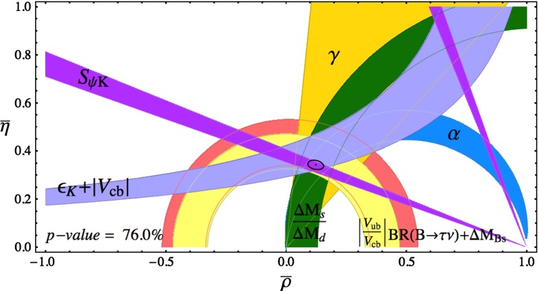
Precision test of the SM mechanism of CP violation in charged-current processes realized through the comparison of the parameters $\overline{\mathit{\rho }}$ and $\overline{\mathit{\eta }}$ determined through various experimental observables and theory inputs from lattice QCD. The experimental inputs are as of September 2013, and the lattice inputs are derived from published results through April 30, 2013; the figure is an update of those in Ref. [1540]

Fig. 42

The box diagram for neutral meson mixing with double $W$ exchange (as in the SM) reduces at low energy to the matrix element of a contact four-quark operator that yields the “bag parameter”

Fig. 43

One of four T-violating asymmetries reported by the BaBar collaboration [1691]

Fig. 44

Top Comparison of the equations of state obtained by the Wuppertal-Budapest group (shaded region) and the HotQCD Collaboration (points). There is still a sizable discrepancy between the results. From [1768]. Bottom The strange quark susceptibilities calculated by the two groups. In the continuum limit, the results agree. From [1136]

Fig. 45

Two scenarios for the phase diagram of QCD for small to moderate baryon chemical potential ${\mathit{\mu }}_B$. In the upper panel, the phase diagram contains a critical point in this region, while in the bottom it does not. From [1764]

Fig. 46

STAR’s measurements of $\mathit{\kappa }{\mathit{\sigma }}^2$, $S\mathit{\sigma }$ and $S\mathit{\sigma }/$Skellam as a function of beam energy, at two different centralities. A Skellam distribution is the difference between two independent Poisson distributions [1803]. Results from $p$+$p$ collisions are also shown. One shaded band is an expectation based on assuming independent proton and antiproton production, and the other shaded band is based on the UrQMD model. From [1803]

Fig. 47

Charged particle pseudorapidity density at midrapidity, $d{N}_{\mathrm{ch}}/d\mathit{\eta }$, per participant as a function of $\sqrt{s_{NN}}$ for $pp$, $pA$ and $AA$. From [1805]

Fig. 48

The direct photon $p_T$ spectrum with the NLO prediction at high $p_T$ and an exponential fit at low $p_T$. From [1812]

Fig. 49

The $p/\mathit{\pi }$ ratio measured for several centrality classes in Pb+Pb collisions relative to $pp$ results at $\sqrt{s_{NN}}=2.76$ TeV. From [1852]

Fig. 50

Top Elliptic flow coefficient $v_2$ as a function of the transverse momenta scaled by the number of constituent quarks in Pb+Pb collisions at $\sqrt{s_{NN}}=2.76$ TeV. Bottom The same data are shown normalized to the polynomial fit to the pion elliptic flow. From [1874]

Fig. 51

The relative increase of the charged particle pseudorapidity density for inelastic collisions having at least one charged particle in $|\mathit{\eta }|<1$, between $\sqrt{s}=0.9$ and 2.36 TeV (open squares) and between $\sqrt{s}=0.9$ and 7 TeV (full squares), is shown for various models. The corresponding ALICE measurements are shown by the vertical dashed and solid lines. The width of the shaded bands correspond to the statistical and systematic uncertainties added in quadrature [1948]

Fig. 52

Charged particle pseudorapidity distributions for $p$+Pb collisions at $\sqrt{s_{NN}}=5.02$ TeV in the laboratory frame. A forward-backward asymmetry between the proton and lead hemispheres is clearly visible with the $\mathrm{Pb}$ remnant going into the direction of positive pseudorapidity. The rcBK (dashed cyan) result is from Ref. [1943]. The IP-Sat result is shown as the dot-dot-dash-dashed black curves. The HIJING2.1 result without (NS, dot-dash-dash-dashed red) and with shadowing ($s_g=0.28$, solid red) and the HIJINGB$\overline{\mathrm{B}}$ result without (dot-dashed magenta) and with shadowing (dotted magenta) are also shown. Finally, the AMPT-def (dot-dash-dash-dashed blue) and AMPT-SM (dot-dot-dot-dash-dash-dashed blue) are given. The ALICE results from Ref. [1950] are given. The systematic uncertainties are shown, the statistical uncertainties are too small to be visible on the scale of the plot. From [1947]

Fig. 53

The charged particle pseudorapidity distributions in Pb+Pb collisions at $\sqrt{s_{NN}}=2.76$ TeV [1951] are compared to model predictions. The horizontal dashed lines group similar theoretical approaches. For the model references see [1951]

Fig. 54

The total multiplicity as a function of center-of-mass energy measured in Au+Au collisions at RHIC (top) and Pb+Pb collisions at the LHC (bottom). The points on the top figure correspond to RHIC data while the dashed curve shows a prediction from the IHQCD scenario [1961]. In the lower figure, the dashed line is a prediction of the same holographic calculation, extended to higher energies. The red point at $2.76$ TeV corresponds to the ALICE measurement [1965], while the other red points are predictions for future LHC runs

Fig. 55

Hierarchies of EFTs for quarkonium at zero temperature (see Sect. 4.1.1 and Ref. [731]) and at finite temperature [–2077]. If $T$ is the next relevant scale after $m_Q$, then integrating out $T$ from NRQCD leads to an EFT called NRQCD${}_{\mathrm{HTL}}$, because it contains the hard thermal loop (HTL) Lagrangian. Subsequently, integrating out the scale $m_{Q}v$ from NRQCD${}_{\mathrm{HTL}}$ leads to a thermal version of pNRQCD called pNRQCD${}_{\mathrm{HTL}}$. If the next relevant scale after $m_Q$ is $m_{Q}v$, then integrating $m_{Q}v$ out from NRQCD leads to pNRQCD. If the temperature is larger than $m_Q{v}^2$, then $T$ may be integrated out from pNRQCD, leading to a new version of pNRQCD${}_{\mathrm{HTL}}$ [2076]. From [2078]

Fig. 56

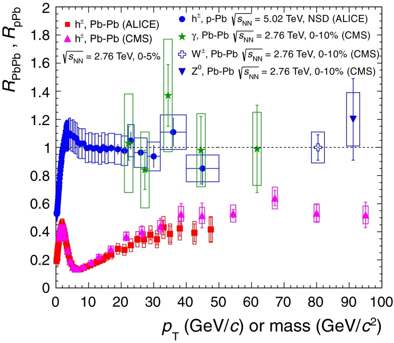
The $R_{AA}$ for charged particles in the 5 % most central Pb+Pb collisions at $\sqrt{s_{NN}}=2.76$ TeV is compared for ALICE and CMS [2104]. The results are also compared to those for $W$and $Z$ bosons as well as isolated photons measured by CMS [1990, 1991, 2107]. The $R_{p\mathrm{Pb}}$ for $p$+Pb collisions at $\sqrt{s_{NN}}=5.02$ TeV measured by ALICE is also shown [2102, 2103]

Fig. 57

Nuclear modification factors $R_{AA}$  at midrapidity versus $p_T$ and centrality, for light and strange particles: pion, kaon, proton, $\mathit{\varphi }$, $\mathrm{\Xi }$ and $\mathrm{\Omega }$. The measurement of pions, kaons and protons at $p_T>3$ GeV/$c$ is in the rapidity window $|y|<0.8$. From [2120]

Fig. 58

The jet $R_{AA}$ over a wide $p_T$ range measured by ALICE and CMS in central Pb+Pb collisions at $\sqrt{s_{NN}}=2.76$ TeV. Data from ALICE [2124] and CMS [2122]; plot from [2125]

Fig. 59

The ratios $R_{CP}^R/R_{CP}^{R=0.2}$ for $R=0.3$, $0.4$ and $0.5$ as a function of jet $p_T$ in the 0–10 % centrality bin. The bars show the statistical uncertainties, the lines indicate fully correlated uncertainties and the shaded boxes represent partially correlated uncertainties between different $p_T$ values. From [2123]

Fig. 60

The $\mathrm{\Delta }\mathit{\varphi }$ dependence of measured jet yield in the 60 $<$ $p_T$ $<$ 80 GeV/c interval for six ranges of collision centrality. The yields are normalized by the total number of jets in the $p_T$ interval. The solid curves are a fit to the data. From [2128]

Fig. 61

The distribution of the mean fractional energy carried by a jet opposite an isolated photon, $x_{\mathrm{J}\mathit{\gamma }}$, in Pb+Pb collisions (closed symbols) compared with PYTHIA “true jet”/“true photon” distributions (yellow histogram) embedded into simulated background heavy-ion events. The rows represent jet cone radii $R=0.2$ (top) and $R=0.3$ (bottom). The columns represent different centralities with increasing centrality from left to right. The error bars represent statistical errors while the gray bands indicate the systematic uncertainties. From [2130]

Fig. 62

The ratio of jet fragmentation functions measured in Pb+Pb and $pp$ collisions in two centrality bins as a function of the scaling variable $\mathit{\xi }=ln(1/z)$, with $z=(p_{\Vert }^{\mathrm{track}}/p^{\mathrm{jet}})$ where $p_{\Vert }^{track}$ is the momentum component of the track along the jet axis, and $p^{jet}$ is the magnitude of the jet momentum. Data from CMS [2134] and ATLAS [2135]; plot from [2136]

Fig. 63

The differential jet shapes, $\mathit{\rho }(r)$, in Pb+Pb and $pp$ collisions determined by CMS shown as a function of the annular regions in the jet cone $r$, in steps of $\mathrm{\Delta }R$ = 0.05. The Pb+Pb data are shown as the filled points while the open circles show the $pp$ reference. In the bottom panel, the ratio of the Pb+Pb to $pp$ jet shapes is shown for annular regions in the jet cone, from the center to the edge of the jet cone radius $R$. The band represents the total systematic uncertainty. From [2138]

Fig. 64

Transverse momentum dependence of the nuclear modification factor $R_{AA}$ for prompt $D$ mesons measured by ALICE as the average of the relevant factors for $D^0$, $D^{+}$, and $D^{\ast +}$ at midrapidity in central Pb+Pb collisions at $\sqrt{s_{NN}}=2.76$ TeV, compared to the $R_{AA}$ of charged hadrons and pions [2144]. The $b$-quark energy loss, via nonprompt $J/\mathit{\psi }$ from $B$-hadron decays by CMS is also shown [2145]. Data from ALICE [2144] and CMS [2145]; plot from [2136]

Fig. 65

Transverse momentum dependence of the ratio of $R_{AA}$ for $D$ mesons to pions [2144]. The data are compared to the following model predictions: Rad (Vitev) and Rad+dissoc (Vitev) [2149, 2150], WHDG [2151], AdS/CFT Drag [2152], CUJET [2153]. From [2154]

Fig. 66

Centrality dependence of the charm and bottom hadron $R_{AA}$ [2159, 2160]. The data are compared to BAMPS [2161], WHDG [2151] and Vitev et al. [2149] model calculations. From [2144]

Fig. 67

The inclusive [2122] and $b$-jet [2145] $R_{AA}$ as a function of $p_T$ in the most central Pb+Pb collisions

Fig. 68

The transverse momentum dependence of $v_2$ for $D$ mesons in the 30–50 % centrality bin relative to that of inclusive charged hadrons. From [2165]

Fig. 69

Azimuthal angular correlations $\mathrm{\Delta }\mathit{\varphi }(\mathrm{HFE},h)$ for $4<p_T^h<6$ GeV$/c$ in 0–8 % (red) and $20\text{--}50\%$ (blue) central Pb–Pb collisions at $\sqrt{s_{NN}}=2.76$ TeV compared to $pp$ collisions at $\sqrt{s}=7$ TeV (black). From [2167]

Fig. 70

The $I_{AA}$ of the near-side $\mathrm{\Delta }\mathit{\varphi }(\mathrm{HFE},\mathrm{hadron})$ correlation in the 0–8 % and 20–50 % most central Pb+Pb collisions [2168]

Fig. 71

Average $D^0$, $D^{+}$, and $D^{\ast }$ $R_{p\mathrm{Pb}}$ [2173] compared with NLO pQCD [139, 2171] and CGC calculations [2174]. From [2173]

Fig. 72

The nuclear modification factor $R_{AA}$ for prompt $J/\mathit{\psi }$, $\mathrm{{\rm Y}}(1S)$ and $\mathrm{{\rm Y}}(2S)$ at midrapidity as a function of the number of participants in Pb+Pb collisions at $\sqrt{s_{NN}}=2.76$ TeV measured in the dimuon channel by the CMS Collaboration. From [2178]

Fig. 73

Inclusive $J/\mathit{\psi }$ $R_{AA}$ in the dimuon channel at forward rapidity in two different centrality bins measured by ALICE [2179]. The curves show transport model calculations [2180]

Fig. 74

Second Fourier coefficient $v_2$ for $J/\mathit{\psi }$ in the 20–60 % centrality range as a function of $p_T$. The ALICE data [2190] are compared with transport model predictions [2191, 2192]. From [2190]

Fig. 75

The nuclear modification factors for inclusive $J/\mathit{\psi }$ production at $\sqrt{s_{NN}}=5.02$ TeV measured by the ALICE Collaboration [2197]. Calculations from several models [1947, 2001, 2198] are also shown. From [2199]

Fig. 76

Top The associated yield per trigger particle in $\mathrm{\Delta }\mathit{\phi }$ and $\mathrm{\Delta }\mathit{\eta }$ for pairs of charged particles with $2<$ $p_T$ $<$ 4 GeV/$c$ for the trigger particle and $1<$ $p_T$ $<$ 2 GeV/$c$ for the associated particle in $p$+Pb collisions at 5.02 TeV for the 0–20 % event multiplicity class. Bottom The same quantity after subtraction of the associated yield obtained in the 60–100 % event class. From [2205]

Fig. 77

The second-order light quark number susceptibility evaluated in two different schemes of resummed perturbation theory (“dimensional reduction-inspired resummation” and HTLpt compared with recent lattice results from the BNL-Bielefeld (BNL-B) and Wuppertal-Budapest (WB) collaborations. From  [2224]

Fig. 78

The conformal trace anomaly, $e-3p$, of SU($N_{\mathrm{c}}$) Yang–Mills theory, normalized by $N_{\mathrm{c}}^2{T}^4$. The points with uncertainties are from lattice calculations [2248], while the yellow line corresponds to the IHQCD prediction [2247]. From [2248]

Fig. 79

The centrality dependence of the correlator $⟨cos({\mathit{\phi }}_{\mathit{\alpha }}+{\mathit{\phi }}_{\mathit{\beta }}-2{\mathrm{\Psi }}_{\mathrm{RP}})⟩$. From [2282]

Fig. 80

Sideward flow excitation function for Au+Au collisions. Data and transport calculations are represented by symbols and lines, respectively [2302]

Fig. 81

The fraction of baryons and leptons in neutron star matter for a RMF [2346] calculation with weak hyperon–hyperon interactions

Fig. 82

Weak charge density ${\mathit{\rho }}_{\mathrm{W}}(\mathrm{r})$ of ${}^{208}\mathrm{Pb}$ that is consistent with the PREX result (solid black line) [2352]. The brown error band shows the incoherent sum of experimental and model errors. The red dashed curve is the experimental (electromagnetic) charge density ${\mathit{\rho }}_{\text{ch}}$

Fig. 83

A given compact star mass (vertical axis) implies an upper bound for the energy density (lower horizontal scale) and the baryon density (upper horizontal scale) in the center of the star. For instance, $M\simeq 2M_{\odot }$ (see middle horizontal dashed line) allows a central baryon density of no more than about 9 times nuclear ground state density. An even heavier star would decrease this upper bound. The solid line that gives this bound is obtained by assuming a “maximally compact” equation of state of the form $P=s(\mathit{ϵ}-{\mathit{ϵ}}_0)$ with $s=1$. Independent of ${\mathit{ϵ}}_0$ one finds ${\mathit{ϵ}}_{\max }{M}_{\max }^2=1.358\times {10}^{16}\mathrm{g}{\mathrm{cm}}^{-3}{M}_{\odot }^2$, which defines the solid line. The various points are calculations within different models and matter compositions. They confirm the limit set by the solid curve and show that equations of state with pure nuclear matter tend to give larger maximal masses than more exotic equations of state. Details can be found in [2436], where this figure is taken from

Fig. 84

Red-shifted effective temperature versus age of the Cas A neutron star: data (encircled star and points with error bars in the zoom-in) and theoretical curves based on the PBF process for various critical temperatures $T_{\mathrm{c}}$ for neutron superfluidity (more precisely the maximal $T_{\mathrm{c}}$, since $T_{\mathrm{c}}$ depends on density). The solid line, also shown in the zoom-in matches the data points, while larger or smaller values for $T_{\mathrm{c}}$ would lead to an earlier or later start of the rapid cooling period. Figure taken from [2449]

Fig. 85

$C_A(\mathit{\lambda })$ for an $L=32a$ lattice with $a=0.085$fm of quenched QCD. From [2565, 2566]

Fig. 86

Infinite volume extrapolation of ${\mathrm{\Lambda }}_{\mathrm{ch}}$. From [2565, 2566]

Fig. 87

Ordinary IPR for zero modes, (8.23). From [2574]

Fig. 88

Fractal dimensions at various cooling stages. The solid line is shown to guide the eye. From [2574]

Fig. 89

Vortex correlation $C_{\mathit{\lambda }}(N_v)$ for overlap eigenmodes on a ${16}^4$ lattice at ${\mathit{\beta }}_{\mathrm{LW}}=3.3$. From [2582]

Fig. 90

${⟨\overline{\mathit{\psi }}\mathit{\psi }⟩}_{{\mathrm{\Lambda }}_{\mathrm{IR}}}/⟨\overline{\mathit{\psi }}\mathit{\psi }⟩$ for an IR cut of ${\mathrm{\Lambda }}_{\mathrm{IR}}=0.5a^{-1}$, plotted against the current quark mass $m$. A large reduction of ${⟨\overline{\mathit{\psi }}\mathit{\psi }⟩}_{{\mathrm{\Lambda }}_{\mathrm{IR}}}/⟨\overline{\mathit{\psi }}\mathit{\psi }⟩\simeq 0.02$ is found in the physical case of $m\simeq 0.006a^{-1}\simeq 5\mathrm{MeV}$. From [2596]

Fig. 91

Inter-quark potential (circles) after removal of low-lying Dirac modes with the IR-cutoff ${\mathrm{\Lambda }}_{\mathrm{IR}}=0.5a^{-1}\simeq 0.4\mathrm{GeV}$ and original potential (squares), apart from an irrelevant constant. From [2596]

Fig. 92

Lattice mass function $M_L(p_{\min }^2)$ for the smallest available momentum $p_{\min }=0.13\mathrm{GeV}$ as a function of the truncation level. On the lower axis the level $k$ is translated to an energy scale. For comparison, the bare quark mass is plotted as a horizontal line. From [2603]

Fig. 93

Influence of the removal of the lowest $k$ modes of the Dirac operator on the masses of chiral partner mesons, the vector meson $\mathit{\rho }$ and axial vector meson $a_1$. From [2603]

Fig. 94

Temperature ($T$) and number of flavors ($N_{\mathrm{f}}$) phase diagram for a generic non-Abelian gauge theory at zero density. In region I, one or more phase boundaries separate a low-temperature region from a high-temperature region. The nature of the phase boundary and which symmetries identify the two phases, in particular the interplay of confinement and chiral symmetry breaking, depend on the fermion representation and the presence or absence of supersymmetry. Region II identifies the conformal window at zero temperature, for $N_{\mathrm{f}}^{\mathrm{c}}<N_{\mathrm{f}}<N_{\mathrm{f}}^{\mathrm{AF}}$, while region III is where the theory is no longer asymptotically free

Fig. 95

NLO determinations of $S$ and $T$, imposing the two WSRs. The approximately vertical (horizontal) lines correspond to values of $M_V$, from $1.5$ to $6.0$ TeV at intervals of $0.5$ TeV ($\mathit{\omega }=M_V^2/M_A^2$: $0.00,0.25,0.50,0.75,1.00$). The arrows indicate the directions of growing $M_V$ and $\mathit{\omega }$. The ellipses give the experimentally allowed regions at 68 % (orange), 95 % (green), and 99 % (blue) CL [2788]

Fig. 96

Scatter plot for the 68 % CL region, in the case when only the first WSR is assumed. The dark blue and light gray regions correspond, respectively, to $0.2<M_V/M_A<1$ and $0.02<M_V/M_A<0.2$ [2788]

Fig. 97

An illustration of the trend of the stability bounds (lower curves) and perturbativity bounds (upper curves) for the SM vacuum from [2813] as a function of the quartic self-coupling of the Higgs field and the Higgs boson mass. The determination of the boundary between the metastable and stable vacuum solution is work in progress, and depends on the experimental uncertainty on the top quark mass, the running strong coupling ${\mathit{\alpha }}_{\mathrm{s}}$, and the Higgs mass itself

Fig. 98

AC conductivity by varying the frequency $\mathit{\omega }$ from the lattice study in [2828] for different values of the inverse coupling $\mathit{\beta }$ in the strong coupling regime

Fig. 99

Typical frequency dependence of the real part (black) and imaginary part (gray) of the fermionic retarded Green function calculated from gauge–gravity duality. We display the 2–2-component in spin space

Fig. 100

Spectral function from [2851] as function of the momentum $k_x/\mathit{\pi }T$ from a gauge–gravity dual model showing non-Fermi liquid behavior. The two curves correspond to different components $R_{11}$ (solid red) and $R_{22}$ (dashed blue) of the fermion matrix in spin space, related by $R_{11}(k_x)=R_{22}(-k_x)$

Fig. 101

Frequency-dependent conductivity for the gauge–gravity superfluid from [2838]. The horizontal axis corresponds to the reduced frequency $\mathit{\omega }/(2\mathit{\pi }T)$. This relativistic model involves a finite isospin density and the new ground state corresponds to a $\mathit{\rho }$ meson condensate. At low frequencies, a gap develops when lowering the temperature. The peaks at higher frequencies above the gap correspond to higher excited modes (similar to the ${\mathit{\rho }}^{\ast }$) in this strongly coupled system

References

-
- J. Beringer et al. (Particle Data Group), Phys. Rev. D 86, 010001 (2012)
- McNeile C, Davies CTH, Follana E, Hornbostel K, Lepage GP. Phys. Rev. D. 2010;82:034512. - PubMed
- Shintani E, Aoki S, Fukaya H, Hashimoto S, Kaneko T, et al. Phys. Rev. D. 2010;82:074505.
- S. Aoki et al. (PACS-CS Collaboration), JHEP 0910, 053 (2009). arXiv:0906.3906
- Blossier B, Boucaud P, Brinet M, De Soto F, Du X, et al. Phys. Rev. Lett. 2012;108:262002. - PubMed
Publication types
LinkOut - more resources
Full Text Sources
Other Literature Sources