High-resolution CMOS MEA platform to study neurons at subcellular, cellular, and network levels

Abstract

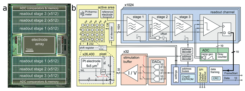
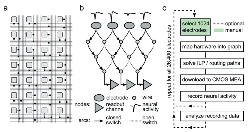
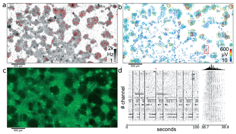
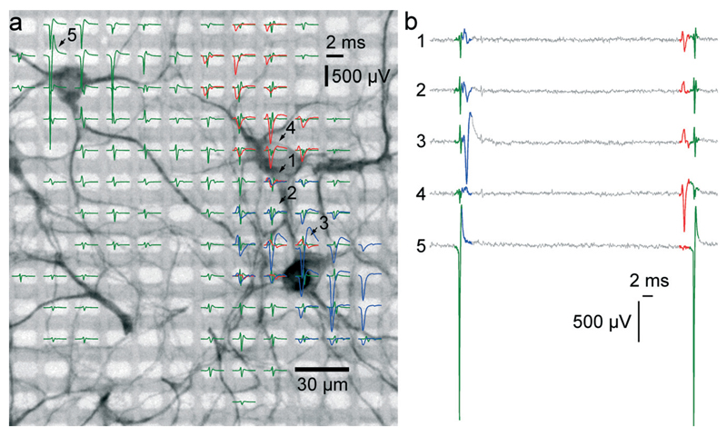
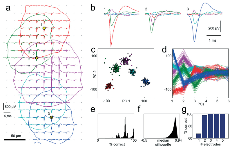
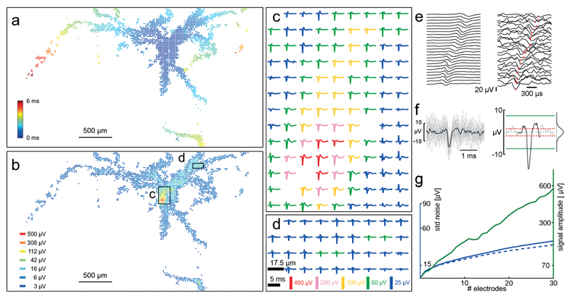
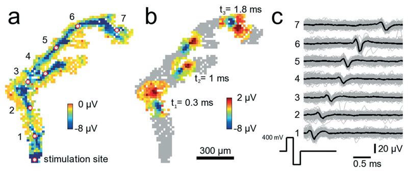
Studies on information processing and learning properties of neuronal networks would benefit from simultaneous and parallel access to the activity of a large fraction of all neurons in such networks. Here, we present a CMOS-based device, capable of simultaneously recording the electrical activity of over a thousand cells in in vitro neuronal networks. The device provides sufficiently high spatiotemporal resolution to enable, at the same time, access to neuronal preparations on subcellular, cellular, and network level. The key feature is a rapidly reconfigurable array of 26 400 microelectrodes arranged at low pitch (17.5 μm) within a large overall sensing area (3.85 × 2.10 mm(2)). An arbitrary subset of the electrodes can be simultaneously connected to 1024 low-noise readout channels as well as 32 stimulation units. Each electrode or electrode subset can be used to electrically stimulate or record the signals of virtually any neuron on the array. We demonstrate the applicability and potential of this device for various different experimental paradigms: large-scale recordings from whole networks of neurons as well as investigations of axonal properties of individual neurons.

Fig. 1. System Architecture.

CMOS MEA system architecture. (a) Micrograph of the CMOS device (10.1 × 7.6 mm²). The 1024 readout channels are arranged at the top and bottom of the 3.85 × 2.10 mm² microelectrode array. The 32 stimulation units (S) are located on the left and right side of the array. (b) Block diagram of the implemented circuitry. A close-up view into the electrode array shows details of one individual pixel including the 9.3 × 5.45 μm² platinum electrode, a two-bit SRAM cell, and two switches.

Fig. 2. Reconfigurable Electrode Array.

(a) Schematic of the wiring in a part of the array. Light gray squares represent electrodes; black squares represent switches controlled by SRAM cells. Buses of 6 horizontal and 6 vertical wires are arranged per row and column. The area highlighted with the red square corresponds to one pixel unit. (b) Simplified mathematical graph showing a drastically reduced subset of the array. Three of the four electrodes picking up neural signals are connected through a set of switches and wires to three readout channels by closing the respective switches. (c) Flow chart of a typical experiment run. After choosing 1024 out of 26 400 electrodes, the hardware is mapped into a mathematical graph representing the array. Within this graph, an integer linear programming (ILP) max-flow min-cost problem is solved, and optimal signal routing paths are determined. The corresponding switch configuration is then downloaded into the CMOS MEA, and neural activity can be recorded. Once the activity on all 26 400 electrodes has been analyzed, best-suited recording electrode candidates are determined so that the final experiment can be performed.

Fig. 3. Network of cortical neurons.

Network of cortical neurons grown over the 3.85 × 2.10 mm² microelectrode array area. (a) Average action potential firing rate as measured by each electrode and displayed on a logarithmic gray-scale between 1 Hz and 2 kHz. Red dots indicate the 1024 electrodes used for recording of the network activity. (b) Representation of all 2000 individual single cells that could be identified through spike sorting the signals of high-density electrode configurations. A circle is drawn around each detectable cell and indicates the level where the amplitude of the electrical signals of a cell footprint exceed −4.5 standard deviations of the electrode noise. The color-coding indicates the maximum amplitude of the most negative peak for each neuronal electrical footprint. The red rectangle indicates the area used for further analysis shown in Fig. 4. (c) Fluorescence image of transfected cells. Transfection ratio was around 5% (according to the manufacturer) of all cells; therefore, only a subset of all cells lights up; clearly visible are clusters of neurons and the tracks of interconnecting neurite bundles. (d) Raster plot of 100 seconds of activity for all 1024 recording channels. The red marker indicates the time period shown in the close up view to the right. Between 38.7 and 38.8 seconds, waves of activity propagate through the network. The histogram at the top shows the number of spikes per time bin.

Fig. 4. Electrical activity superimposed to a MAP2 staining of the neurons.

(a) The electrical activity of three neurons is superimposed to a fluorescence image of a MAP2 staining of the cell culture in the respective area. Spike-triggered averages of signals from 3 different neurons over 50 trials are drawn in green, red and blue. Averaged traces are only displayed for electrodes with a peak-to-peak signal amplitude exceeding 50 μV. The activity of a single cell can be recorded on fairly distant electrodes. Particularly, the green traces exhibit signals of very large amplitudes (almost 3 mV peak-to-peak), and putative axonal signals can be seen at electrodes at more than 180 μm distance from the soma. The red set of signal traces exhibits the largest negative peak value in the 4th row, 9th column and features signals with negative peaks in the first row and signals with positive peaks in the 8th row. (b) Sixty milliseconds of raw data as recorded on the five electrodes marked with arrows and numbers in (a). At least three individual spikes can be identified in this period. The activities of the single cells can be recorded through multiple electrodes.

Fig. 5. Single-cell resolution.

The electrical activity of five neurons has been identified and spike-sorted with 209 electrodes. Subsequently, the performances of all combinations of selecting 3 out of 209 electrodes were analyzed in terms of correctly classified APs. Refer to text for a detailed discussion of the procedure. (a) Spike-triggered averages of five identified neurons with overlapping electrical footprints. For each neuron, a circle is drawn where the amplitude of their electrical signal exceeds a threshold of 4.5 standard deviations of the noise level. Black-yellow circles indicate the three electrodes yielding best sorting performance. (b) Spike-triggered average waveforms recorded with the three electrodes marked in (a). (c) Principal component (PC) projection of 500 AP waveforms recorded with the three electrodes marked in (a). The PC projection is used for clustering. (d) First six PCs of all 500 AP waveforms. Color coding of the neurons is identical for all subfigures. (e) Distribution of performances for all 1.45 million tested electrode combinations. A considerable fraction yields more than 95% correct classifications. (f) Distribution of medians of the silhouette coefficients for all 1.45 million tested electrode combinations for the clustered waveforms as in (c). (g) Comparison of the best achievable spike-sorting performance for different numbers of electrodes. With just one electrode, only about 65% of all APs can be correctly classified. With three electrodes and more, the performance saturates at 100%, thus three electrodes chosen at suitable spots are sufficient to reliably record and distinguish the signals from the five neurons displayed in (a). The supplementary material contains more figures that show the analysis for one, two, four and five out of 209 selected electrodes (see ESI,† SF1_a–SF1_e).

Fig. 6. Axonal arbors.

Identified axonal arbor of a single cell revealing subcellular features up to more than 2 mm distance from the cell body. (a) All electrodes capturing activity attributed to a single neuron. Color-coding indicates the time of arrival of the AP at the respective electrode. It takes 6 ms for the AP to arrive at the left-most visible axonal segment. A video showing the AP propagation down the axonal arbor is available as ESI† Video SM1. (b) The same neuron and electrodes as in (a), this time showing the amplitude of the most negative peak on a logarithmic color-scale. Its putative soma is inside the box indicated with (c). (c) And (d) spike-triggered averages (30 to 50 averages) of the electrical footprint from two areas of the array as indicated in (b). The scale bars of (d) apply to the signals in (c) and (d). (e) Left: 25 traces from electrodes that detect axonal signals. Spike-triggered averaging (50 APs) reduces noise. Right: traces from the same electrodes showing a single axonal AP hidden in the noise. Red dots indicate the timing of the negative peak. (f) Left: all 25 recording traces of one axonal AP overlaid and aligned in time with respect to the negative peak. Right: spatial averaging of traces aligned in time with respect to the negative peak from multiple neighbored electrodes that detect axonal signals improves axonal AP detectability. The Gaussian-like distribution of the noise is shown, and dashed red lines indicate one standard deviation. Green lines indicate 4.5 standard deviations, the detection threshold. (g) The signal amplitude (green curve, right ordinate) scales linearly with an increasing number of electrodes (#electrodes), whereas the noise floor (blue curve, left ordinate) scales with a square root function. The dashed blue curve indicates the scaling of uncorrelated noise. When summing signals from more than four electrodes, the signal amplitude is more than 4.5 times larger (70 μV) than the standard deviation of the noise (15 μV), so that the signals can be considered detectable. See text for a more detailed discussion.

Fig. 7

Tracking of stimulated signals in axonal arbors. 841 electrodes below an axonal arbor record the stimulation-induced axonal propagation of an AP. A video showing the propagating AP is available as ESI† Video SM3. (a) The site at the bottom denoted stimulation site has been stimulated 200 times with biphasic 300 mV voltage pulses at 300 ms inter-stimulus intervals. Each square shows the average AP minimum value on a clipped color scale over the 200 trials for each recorded electrode within 3 ms after stimulation. The red circles with white fillings indicate electrodes for which voltage traces are shown in (c). Close to the electrode indicated with 3, the axon splits into two different branches. (b) Same neuron and electrodes as in (a). This time, the propagating AP is shown at three different time points, t₁ = 0.3, t₂ = 1.0 and t₃ = 1.8 ms after stimulation occurred. At t₂, the AP has already passed the branch point such that the AP can be seen in both branches. (c) Voltage traces from the 7 electrodes marked with the red-white circles in (a). Shown are voltage traces for single trials (gray) and the median over all trials (black).

Fig. 8. Electrode impedance measurements.

Shown are the capacitances of 300 randomly selected bright Pt and Pt-black electrodes based on impedance measurements at 1 kHz. The capacitances are plotted on a logarithmic scale. The capacitances of Pt-black electrodes are about 50 times larger than those of the bright Pt electrodes. The distribution shown in green indicates the capacitances for 300 randomly selected electrodes after 5 months of culturing cells on top of them.

References

1. Alivisatos AP, Andrews AM, Boyden ES, Chun M, Church GM, Deisseroth K, Donoghue JP, Fraser SE, Lippincott-Schwartz J, Looger LL. ACS Nano. 2013;7:1850–1866. - PMC - PubMed
1. Marblestone AH, Zamft BM, Maguire YG, Shapiro MG, Cybulski TR, Glaser JI, Amodei D, Stranges PB, Kalhor R, Dalrymple DA, Seo D, et al. Front Comput Neurosci. 2013;7:137. doi: 10.3389/fncom.2013.00137. - DOI - PMC - PubMed
1. Gerhard F, Kispersky T, Gutierrez GJ, Marder E, Kramer M, Eden U. PLoS Comput Biol. 2013;9:e1003138. - PMC - PubMed
1. Sjöström PJ, Rancz EA, Roth A, Häusser M. Physiol Rev. 2008;88:769–840. - PubMed
1. Zhang W, Linden DJ. Nat Rev Neurosci. 2003;4:885–900. - PubMed
Publication types