Behavioral responses to a repetitive visual threat stimulus express a persistent state of defensive arousal in Drosophila

Abstract

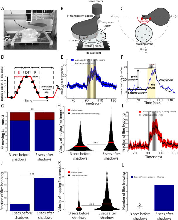
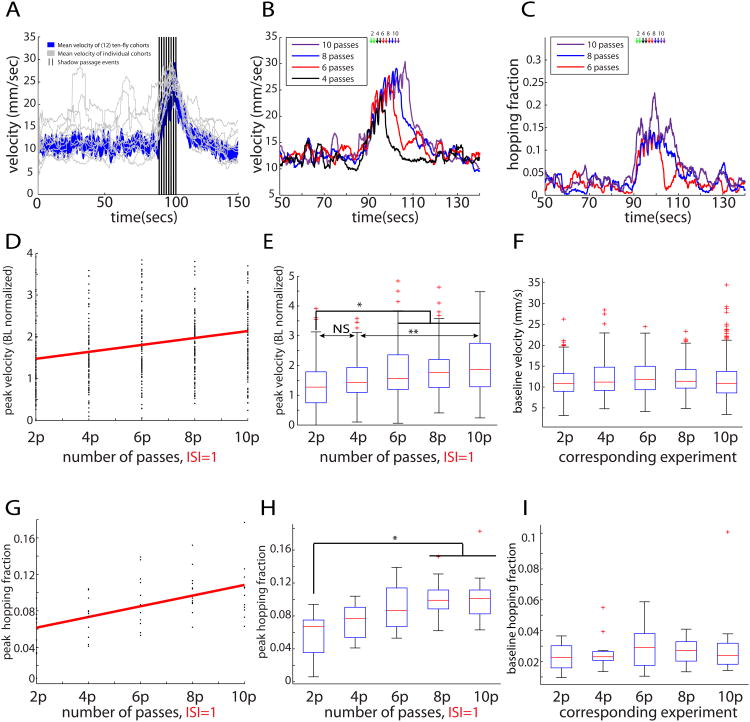
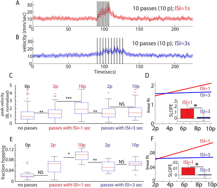
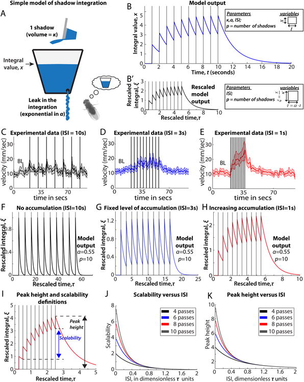
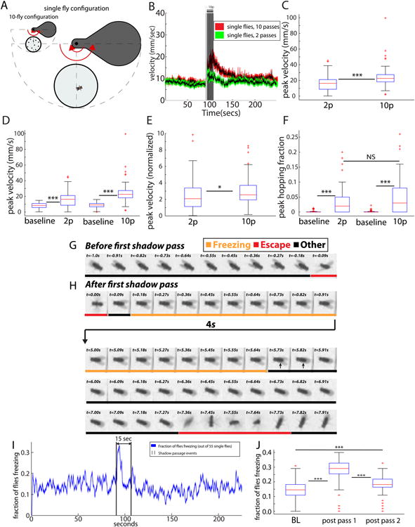
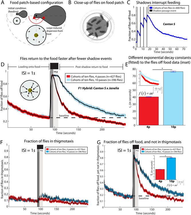
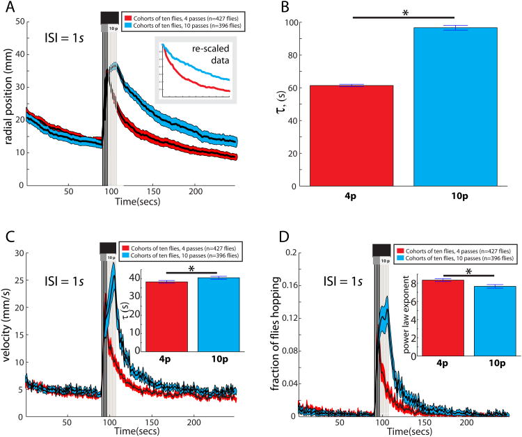
The neural circuit mechanisms underlying emotion states remain poorly understood. Drosophila offers powerful genetic approaches for dissecting neural circuit function, but whether flies exhibit emotion-like behaviors has not been clear. We recently proposed that model organisms may express internal states displaying "emotion primitives," which are general characteristics common to different emotions, rather than specific anthropomorphic emotions such as "fear" or "anxiety." These emotion primitives include scalability, persistence, valence, and generalization to multiple contexts. Here, we have applied this approach to determine whether flies' defensive responses to moving overhead translational stimuli ("shadows") are purely reflexive or may express underlying emotion states. We describe a new behavioral assay in which flies confined in an enclosed arena are repeatedly exposed to an overhead translational stimulus. Repetitive stimuli promoted graded (scalable) and persistent increases in locomotor velocity and hopping, and occasional freezing. The stimulus also dispersed feeding flies from a food resource, suggesting both negative valence and context generalization. Strikingly, there was a significant delay before the flies returned to the food following stimulus-induced dispersal, suggestive of a slowly decaying internal defensive state. The length of this delay was increased when more stimuli were delivered for initial dispersal. These responses can be mathematically modeled by assuming an internal state that behaves as a leaky integrator of stimulus exposure. Our results suggest that flies' responses to repetitive visual threat stimuli express an internal state exhibiting canonical emotion primitives, possibly analogous to fear in mammals. The mechanistic basis of this state can now be investigated in a genetically tractable insect species.

Figure 1

Introduction to Repetitive Shadow-Induced Arousal (ReSA). (A-B) Shadow paddle apparatus. (C) Motion of the shadow paddle. (D) Control of swipe delivery. Dwell time (DT) and inter-shadow interval (ISI) control, respectively, how long the paddle remains at θ=π and θ=0. (E) Canonical ReSA curve for a cohort of ten male flies, with SEM envelopes. Shadow passes separated by an ISI of 1 second (vertical bars, black) cause an increase in velocity (yellow shaded region), which persists following stimulus cessation, and then decays back to baseline. (F) Illustration of baseline and peak height, as well as the three phases (“baseline,” “rise phase,”and “decay phase”). (G) Proportion of flies moving in the 3s before and after the shadow (**,Chi-square test). (H) Velocities of moving flies, in the 3s before and after the shadows (***, Kruskal-Wallis test). (I) Fraction of flies hopping over time (black), with SEM envelope (red). (J) Fraction of flies hopping increases relative to baseline (***,Chi-square test). (K) Velocity of hopping flies increases relative to baseline (***, Kruskal-Wallis test). Sample size for panels (E-K) is n=120 flies. (L) Number of flies freezing for ≥10 frames. Asterisks represent p-values, where (*), (**), and (***) denote, respectively, p<.05,p<.01, and p<.001. We use α=.05.

Figure 2

For ISI=1s, peak velocity scales with swipe number. (A) Mean velocity across 12 ten-fly cohorts (blue), with sample trajectories (grey; 1 per cohort) in response to shadows (black). (B) The number of shadow passes (back-and-forth), whether 4 (black), 6 (red), 8 (blue), or 10 (purple), alters the response's peak velocity. (C) The fraction of flies jumping increases with pass number: 6 (red), 8 (blue), or 10 (purple). (D) Linear regression (red) for the response's peak height, when flies receive 2-10 passes (*significantly different from zero, see bottom of legend). (E) Slope is non-zero (Kruskal-Wallis test), as confirmed by pair-wise tests (see bottom of legend); see Figure S2A. Peak velocity, normalized to baseline, for flies receiving 2-10 passes with ISI=1s. (F) Baselines for data in (E) are not different from each other (Kruskal-Wallis test). (G) A linear regression (red) with positive slope (*,see bottom of legend) for the fraction of hopping flies receiving 2-10 passes. (H) Pair-wise tests (see bottom of legend) confirm a monotone increasing trend in the median values. (I) Baseline hopping fractions are not different from each other (Kruskal-Wallis test). Total sample sizes for the 2-10 pass experiments are, respectively, 110, 109, 108, 120, and 119 flies. Cohort sizes were 8-10 flies each. Panels (A-I) re-use data from Figures 1E-K for purposes of analysis and direct comparison. Unless otherwise indicated, in this and all subsequent main and supplemental figures pair-wise tests are Bonferroni-corrected post-hoc Mann-Whitney U tests following significant differences determined by Kruskal-Wallis 1-way ANOVA. Asterisks represent p-values, where (*),(**), and (***) denote, respectively, p<.05,p<.01, and p<.001. We use α=.05. Slopes from (D) and (G)differ from zero (*) because their 95% CI's exclude zero.

Figure 3

Scalability in ReSA depends on ISI value. (A) Response to 10 passes (black bars) with ISI=1s (red), or (B) ISI=3s (blue). (C) Peak velocity is greater (***) following p=10 versus p=2 when ISI=1s (red), but not when ISI=3s (blue). (D) Linear fits to the peak velocity versus p for ISI=1s (red) and ISI=3s (blue). (D, inset) Slopes are significantly different (*, see bottom of legend). Slope for ISI=1s is positive, but for ISI=3s, it is indistinguishable from zero (*, see bottom of legend). (E) Hopping fraction is greater for p=10 versus p=2 when ISI=1s (*), but not when ISI=3s. (F) Linear fits to peak hopping fraction versus p, for ISI=1s (red) and ISI=3s (blue). (F, inset) Slope values. Slope for ISI=1s is positive (*, see bottom of legend), but for ISI=3s, it is indistinguishable from zero. In ISI=1s groups, for p=2…10, sample sizes are, respectively, 110, 109, 108, 120, and 119 flies. For the ISI=3s groups, for p=2…10, sample sizes are, respectively, 100, 110, 100, 110, and 118 flies. For ISI=1s, data in (C-F) are re-used from Figure 2 for comparative purposes. Asterisks represent p-values, where (*), (**), and (***) denote, respectively, p<.05,p<.01, and p<.001. Slopes from (D) and (F) differ (*), because their 95% CI's do not overlap. Slopes for ISI=1 have 95% CI's that exclude zero; hence they differ (*) from zero.

Figure 4

A leaky integrator of shadow exposure. (A) Cumulative shadow integral is analogous to the water level in a reservoir. Shadows (cups of water) fill the reservoir, whereas a slow leak drains the reservoir (B) Model output (blue), with shadow passes (black lines). Model parameters are: κ, the fill rate; α, the leak rate; pass number, p, which is the number of shadows received; and the ISI. Variables (inset) are time, t, and the reservoir's fill level, x. (B′) Rescaled model output (black), which eliminates redundant parameters to simplify analysis (see Supplemental Experimental Procedures). The parameters for the rescaled model are: pass number, p, and the ISI. Variables (inset) are τ = t·α, and $\xi =\frac{x}{\kappa }$. See Supplementary Experimental Procedures for detailed explanation. (C-E) Experimental time series data for ISI=10s, 3s, and 1s. (F-H) Model output (α =.55). (F) When ISI=10s, the reservoir completely empties between passes, as in (C). (G) When ISI=3s, the integral saturates after only a few passes, as in (D). (H) When ISI=1s, the integral increases, as in (E). (I) Diagram illustrating scalability and peak height definitions (see Supplemental Experimental Procedures). (J) Scalability versus pass number p and ISI. (K) Peak height versus p and ISI. Data from (D-E) are from Figure 3A-B. Sample sizes for (D-F) are 105, 118, and 119 flies.

Figure 5

(A) Single-fly ReSA assay. (B) Time course for single fly velocities. For pass number p=10 (red envelope, black curve), the peak velocity is greater and it persists longer than for p=2 (green envelope, black curve). (C) Peak velocity for p=10 is significantly greater than for p=2 (***,Kruskal-Wallis test). (D) Peak velocities differ from baseline, and increase with p (***). (E) Peak velocity for p=10 is still greater than p=2 when normalized to baseline (*, Kruskal-Wallis test). (F) Peak hopping fraction for p=10 trends towards being greater than p=2; both values differ significantly from baseline (***). (G) Kymograph prior to the first pass (orange for freezing, red for escape, and black for other). (H) Kymograph following first shadow pass. Most time is spent freezing (orange label). Long arrow from t=.91 to t=5.00 s represents 4-seconds of freezing. After freezing, the fly escapes (red label). (I) Proportion of flies freezing vs time (see experimental procedures). Proportion freezing spikes following the first shadow (J) Shadow-induced elevation in the freezing rate (***). For panels B-F, the sample size is n=81 for each condition. Sample sizes for panels I-J are n=55 single flies. See also Movie S2.

Figure 6

(A) Food-based version of the assay, with a central food cup at the arena's center. (B) Flies feeding on the food cup. (C) Shadow passes cause starved Canton S flies (n=810 flies in 81 cohorts) to leave the food, with more flies leaving at each successive pass. (D) Despite identical “loading onto food” kinetics (red and blue enveloped curves), flies return to the food faster when they receive fewer shadows (pass number p=4, black vs p=10, grey; ISI=1s). The “post-shadow return to food” region of the plot shows different kinetics of return for the two different pass treatment groups. Flies receiving 4 passes drop below baseline, whereas the 10-pass cohorts never reach baseline. The case p=4 has a steeper decay function than the case p=10 (E), which is statistically significant (*, see bottom of legend). (F) Thigmotaxis is rare in whether p=4 or p=10. (G) Subset of flies off the food, and not in thigmotaxis, also shows a statistically significantly steeper (*, see bottom of legend) decay for p=4 than for p=10, suggesting that thigmotaxis is not responsible for the decay rate difference. Sample sizes for panels (D-G) are all n=46 experiments for p=4 and for p=10. Decay constants in (E) and (G) are different (*) because their 95% CI's do not overlap.

Figure 7

(A) Radial dispersal of flies from food. Flies receiving 10 passes of the shadow are initially slightly further from the center than flies that receive 4 passes of the shadow, but the return kinetics are different based on rescaling (inset) or (B) an exponential fit to the data. (B) Tau values for the p=10 and p=4 pass conditions (*significantly different; see bottom of legend). (C) When p=10 (blue envelope), there is a higher peak velocity, and slower decay (*, see bottom of legend), than when p=4 (C, inset). (D) Hopping frequency return to baseline more quickly (*, see bottom of legend;based on a power-law fit to the decay region of the function; D, inset) when flies receive 4 vs. 10 passes of the shadow. Sample sizes for panels (A-D) are all n=46 experiments for 4 pass scenario; n=46 experiments for the 10 pass scenario. Each experiment contains 7-10 flies. Panels in Figure 7 are computed from the same dataset as panels in Figures 6D-G. Decay constants in (B), (C) and (D) differ (*) because their 95% CI's do not overlap.

References

1. Simon HA. Motivational and Emotional Controls of Cognition. Psychol Rev. 1967;74:29–&. - PubMed
1. Sloman A, Croucher M. Why robots will have emotions 1981
1. Anderson DJ, Adolphs R. A framework for studying emotions across species. Cell. 2014;157:187–200. - PMC - PubMed
1. Darwin C. The expression of the emotions in man and animals. London: J. Murray; 1872.
1. Oatley K, Johnson-Laird PN. Towards a cognitive theory of emotions. Cogn emot. 1987;1:29–50.
Publication types