An Integration Factor Method for Stochastic and Stiff Reaction-Diffusion Systems

Abstract

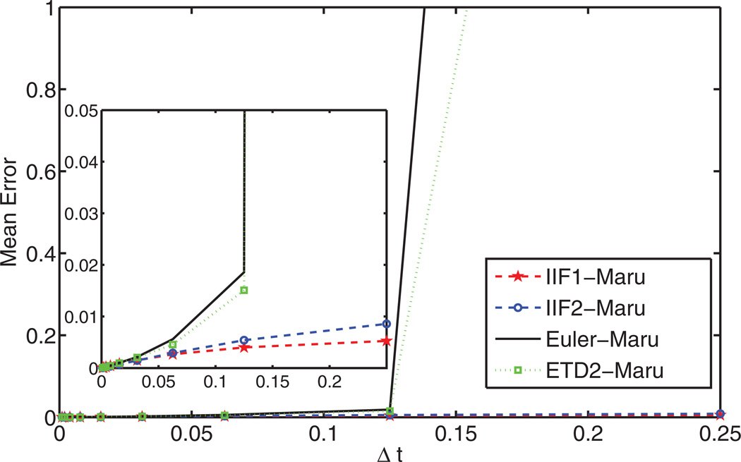
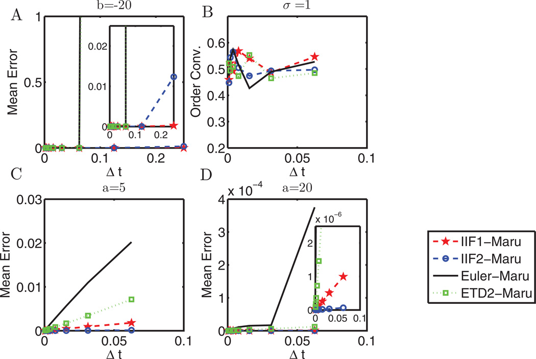
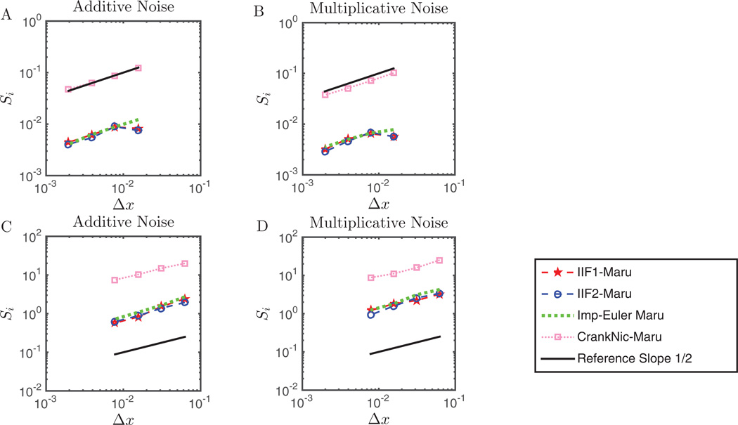
Stochastic effects are often present in the biochemical systems involving reactions and diffusions. When the reactions are stiff, existing numerical methods for stochastic reaction diffusion equations require either very small time steps for any explicit schemes or solving large nonlinear systems at each time step for the implicit schemes. Here we present a class of semi-implicit integration factor methods that treat the diffusion term exactly and reaction implicitly for a system of stochastic reaction-diffusion equations. Our linear stability analysis shows the advantage of such methods for both small and large amplitudes of noise. Direct use of the method to solving several linear and nonlinear stochastic reaction-diffusion equations demonstrates good accuracy, efficiency, and stability properties. This new class of methods, which are easy to implement, will have broader applications in solving stochastic reaction-diffusion equations arising from models in biology and physical sciences.

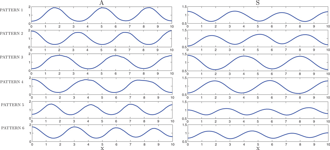
Keywords: IIF-Maruyama; Integration Factor method; Stochastic reaction-diffusion systems; activator-susbtrate system; patterns.

Figure 1

The stability regions of both IIF-Maruyama methods described in Eqs.(17) and (18) for multiplicative noise. The stability region lies below the corresponding colored curve. The desired absolute stability region is the region inside the square with dashed-border.

Figure 2

Comparison of stability regions of the following methods: IIF1-Maruyama, IIF2-Maruyama, Euler Maruyama, RK2-Maruyama, and ETD2-Maruyama used to solve Eq.(19) with multiplicative noise. The stability region for each method is shaded blue. The ideal absolute stability region is the region inside the dashed box.

Figure 3

Enlarged version of Figure 2. In this figure, the stability regions are enlarged for the following methods: IIF1-Maruyama, IIF2-Maruyama, and ETD2-Maruyama. The stability region for each method is shaded blue. The ideal absolute stability region is the region inside the dashed box.

Figure 4

Comparison of the mean errors 𝔼|U_Δt −U_Δt/2| of the numerical solutions to Eq.(19) with additive noise obtained from the following methods: IIF1-Maruyama, IIF2-Maruyama, Euler Maruyama, and ETD2-Maruyama, when the reaction term is heavily stiff. The inserted figure shows the mean error comparison between different methods in more detail. The parameter values are as followed: a = 1, b = −10, and σ = 0.1.

Figure 5

Comparison of the orders of convergence of the following methods: IIF1-Maruyama, IIF2-Maruyama, Euler Maruyama, and ETD2-Maruyama used to solve Eq.(19) with additive noise. Subplots A and B represent the orders of convergence of all the methods in the scenario that the noise amplitude is relatively large compared to the magnitudes of the diffusion and reaction terms, whose values are fixed to be a = 0.1 and b = −1. Subplots C and D represent the scenario where the magnitude of the diffusion term is great compared to those of the reaction and noise terms, whose values are fixed to be σ = 0.1 and b = −1.

Figure 6

Comparison of the mean errors and orders of convergence between the following methods: IIF1-Maruyama, IIF2-Maruyama, Euler Maruyama, and ETD2-Maruyama, used to solve Eq.(19) with multiplicative noise. Subplot A is the comparison of the mean errors 𝔼|U_n − U(τ)| of the numerical solutions when the reaction term is heavily stiff. The parameters used here are a = 1, b = −20, and σ = 0.1. In the scenario that the noise amplitude is relatively large compared to the magnitudes of the diffusion and reaction term, all methods display similar orders of convergence, as seen in subplot B. The parameter values for this subplot are a = 0.1, b = −0.02, and σ = 1. Finally, subplots C and D compare the mean errors 𝔼|U_n − U(τ)| of the numerical solutions when the diffusion term is dominant using fixed parameters σ = 0.1 and b = −2. The time span for the simulations in subplot A is one and the time span used in subplots B–D is one-half. For subplots A and D, the inserted images show the mean errors of each method in more detail.

Figure 7

Comparison of the values ${\{S_i\}}_{i=1}^4$ from Eq.(47) and orders of convergence of the following methods: IIF1-Maruyama, IIF2-Maruyama, Implicit-Euler Maruyama, and Crank-Nicolson Maruyama used to solve Eq.(44) with both additive and multiplicative noises in the scenario where the reaction term is heavily stiff. Subplots A and B show the plots of ${\{S_i\}}_{i=1}^4$ of all the methods when the reaction term b = −10. Subplots C and D display plots of ${\{S_i\}}_{i=1}^4$ of all the methods when b = −50. For all the subplots, the values of the reaction and noise terms are fixed to be a = 1 and σ = 0.1. In subplots A and B, the time frame is chosen to be t ∈ [0, 0.125] and for the remaining two subplots, t ∈ [0, 0.025]. Also, each plot contains the reference line of slope one-half for the purpose of order of convergence comparison.

Figure 8

Comparison of the values ${\{S_i\}}_{i=1}^4$ from Eq.(47) and orders of convergence of the following methods: IIF1-Maruyama, IIF2-Maruyama, Implicit-Euler Maruyama, and Crank-Nicolson Maruyama used to solve Eq.(44). Subplots A and B are the plots of ${\{S_i\}}_{i=1}^4$ of all the methods when the diffusion term is stiff. The values of the diffusion, reaction, and noise terms are fixed to be a = 20, b = −1, and σ = 0.1 for all subplots. Subplots C and D display plots of ${\{S_i\}}_{i=1}^4$ of all the methods when the noise term assumes a large value. For these subplots, the values of the diffusion, reaction, and noise terms are fixed to be a = 2, b = −1, and σ = 1. In this figure, all the simulations are run for 0.125 time units. Also, each plot contains the reference line of slope one-half for the purpose of order of convergence comparison.

Figure 9

The six different combinations of steady-state patterns for long-term solutions A and S to the one-dimensional stochastic system in Eqs.(54) and (55). The values for the noise coefficients are ε_S = 0.01 and ε_A = 0.005.

Figure 10

One of the final patterns obtained for long-term solutions A and S when solving the two-dimensional stochastic system in Eqs.(54) and (55). The values for the noise coefficients are ε_S = 0.01 and ε_A = 0.005.

References

1. Kondo S, Miura T. Reaction-diffusion model as a framework for understanding biological pattern formation. Science. 2010;329:1616–1620. - PubMed
1. Wilkinson DJ. Stochastic modeling for quantitative description of heterogeneous biological systems. Nat Rev Genet. 2009;10:122–133. - PubMed
1. Wang L, Xin J, Nie Q. A critical quantity for noise attenuation in feedback systems. PLoS Comput Biol. 2010;6:e1000764. - PMC - PubMed
1. Lawson MJ, Drawerr B, Khammash M, Petzold L, Yi T. Spatial stochastic dynamics enable robust cell polarization. PLoS Comput Biol. 2013;9 - PMC - PubMed
1. Zhang L, Radtke K, Zheng L, Cai AQ, Schilling TF, Nie Q. Noise drives sharpening of gene expression boundaries in the zebrafish hindbrain. Molecular Systems Biology. 2012;8 - PMC - PubMed