Using Genome-scale Models to Predict Biological Capabilities

Abstract

Constraint-based reconstruction and analysis (COBRA) methods at the genome scale have been under development since the first whole-genome sequences appeared in the mid-1990s. A few years ago, this approach began to demonstrate the ability to predict a range of cellular functions, including cellular growth capabilities on various substrates and the effect of gene knockouts at the genome scale. Thus, much interest has developed in understanding and applying these methods to areas such as metabolic engineering, antibiotic design, and organismal and enzyme evolution. This Primer will get you started.

Figure 1. Network reconstruction

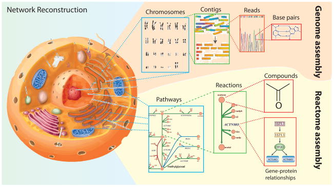
A. An organism’s reactome can be assembled in a way that is analogous to DNA sequencing assembly. From right to left: first the interacting compounds must be identified. Then, the reactions acting on these compounds are tabulated and the protein that catalyzes the reaction and the corresponding open reading frame is identified in the organism of interest. These reactions are assembled into pathways that can be laid out graphically to visualize a cell’s metabolic map at the genome-scale. Several tools for reactome assembly and curation exist including the COBRA Toolbox (Ebrahim et al., 2013; Schellenberger et al., 2011b), KEGG (Kanehisa et al., 2014), EcoCyc (Keseler et al., 2013), ModelSeed (Henry et al., 2010b), BiGG (Schellenberger et al., 2010), Rbionet (Thorleifsson and Thiele, 2011), Subliminal (Swainston et al., 2011), Raven toolbox (Agren et al., 2013) and others.

Figure 2. Formulation of a computational model

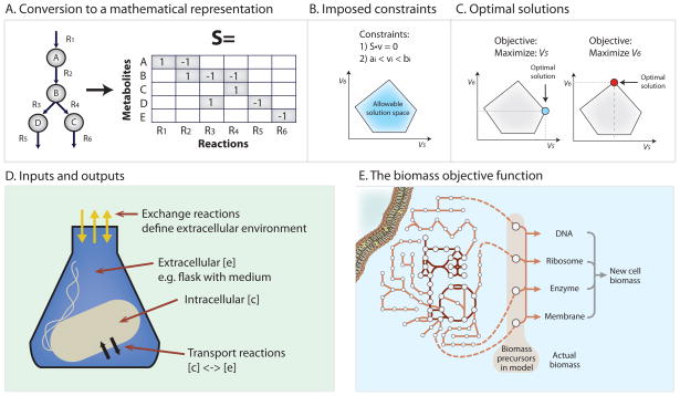
A. After the metabolic network has been assembled it must be converted into a mathematical representation. This conversion is performed using a stoichiometric (S) matrix where the stoichiometry of each metabolite involved in a reaction is enumerated. Reactions form the columns of this matrix and metabolites the rows. Each metabolite’s entry corresponds to its stoichiometric coefficient in the corresponding reaction. Negative coefficient substrates are consumed (reactants), and positive coefficients are produced (products). Converting a metabolic network reconstruction to a mathematical formulation can be achieved with several of the toolboxes listed in Supplemental Table 1. B. Constraints can be added to the model such as 1) enforcement of mass balance and 2) reaction flux (v) bounds. The blue polytope represents different possible fluxes for reactions 5 and 6 consistent with stated constraints. Those outside the polytope violate the imposed constraints and are thus ‘infeasible.’ C. Constraint-based models predict the flow of metabolites through a defined network. The predicted path is determined using linear programming solvers and termed Flux Balance Analysis (FBA). FBA can be used to calculate the optimal flow of metabolites from a network input to a network output. The desired output is described by an objective function. If the objective is to optimize flux through reaction 5, the optimal flux distribution would correspond to the levels of flux 5 and flux 6 at the blue point circled in the figure. The objective function can be a simple value or draw on a combination of outputs, such as the biomass objective shown in Fig 2E. It is important to note that alternate optimal flux distributions may exist to reach the optimal state as discussed in Figure 4C. D. Once a network reconstruction is converted to a mathematical format, the inputs to the system must be defined by adding consideration of the extracellular environment. Compounds enter and exit the extracellular environment via ‘exchange’ reactions. The GEM will not be able to import compounds unless a transport reaction from the external environment to the inside of the cell is present. E. In addition to exchange reactions, the biomass objective function acts as a drain on cellular components in the same ratios as they are experimentally measured in the biomass. In FBA simulations the biomass function is used to simulate cellular growth. The biomass function is composed of all necessary compounds needed to create a new cell including DNA, amino acids, lipids and polysaccharides. This is not the only physiological objective that can be examined using COBRA tools.

Figure 3. Using models for qualitative predictions and iterative improvement

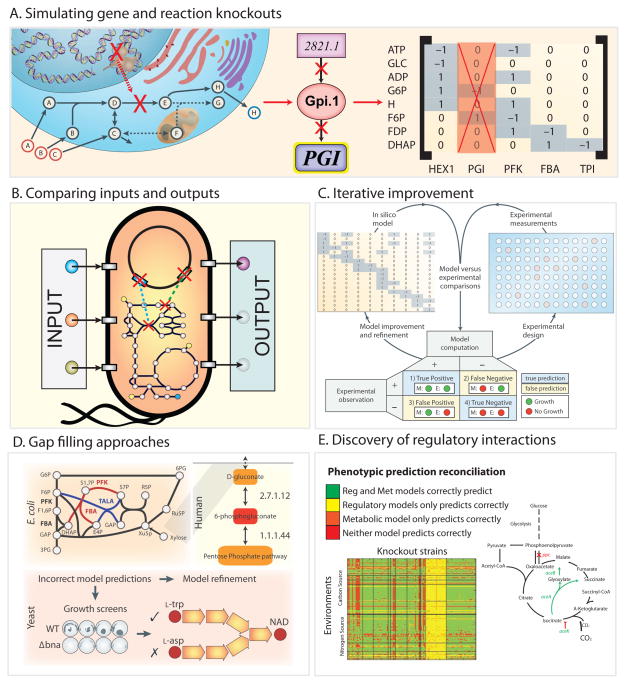
A. Each reaction in the network is linked to a protein and encoding gene through the gene-protein-reaction (GPR) relationship. Because each reaction in the network corresponds to a column in the stoichiometric matrix, simply removing the column association with a particular reaction can simulate gene knockouts. Thus, multiple KO simulations can be performed. For example, it is easy to delete every pairwise combination of 136 central carbon metabolic E. coli genes to find double gene knockouts that are essential for survival of the bacteria. B. The simplicity of altering inputs to change cellular growth environments and removing genes in silico allows one to perform simulations in millions of experimental conditions quickly. Even on a modest laptop computer a single FBA calculation runs in a fraction of a second, thus simulating the effect of all gene knockouts in E. coli central metabolism can be run in less than 10 seconds. C. Incorrect model predictions are an opportunity for biological discovery because they highlight where knowledge is missing. Targeted experiments can be performed to discover new content that can then be added back to a model to improve its predictive accuracy. Missing model content can be discovered using automated approaches known as ‘gap-filling’ (Orth and Palsson, 2010a) that query a universal database of potential reactions to restore in silico growth to a model. D. Gap-filling approaches have been used to discover new metabolic reactions in several organisms. E. coli: Two new functions for two classical glycolytic enzymes phosphofructokinase (PFK) and fructose-bisphosphate aldolase (FBA) were discovered (red) (Nakahigashi et al., 2009a). Human: Gluconokinase (EC 2.7.1.12) activity was discovered based on the known presence of the metabolite 6-phosphogluconolactonate in the human reconstruction (Rolfsson et al., 2011b) (red). Yeast: Automated model refinement suggested modifications in the NAD biosynthesis pathway. Experiments demonstrated that a parallel pathway from aspartate thought to exist in yeast was not present (Szappanos et al., 2011). E. False positive predictions can be reconciled by adding regulatory rules derived from high throughput data (Covert et al., 2004), for example, a recent study was able to reconcile 2,442 false model predictions from the E. coli GEM by updating the function of just 12 genes (Barua et al., 2010). Additionally, a false positive growth inconsistency in the metabolic model of S. Typhimurium was reconciled by updating regulatory rules for the iclR gene product’s transcriptional repression of aceA encoding isocitrate lyase. Transcriptional repression can also often be relieved via adaptive laboratory evolution. Such evolution drives experimental phenotypes to achieve model predictions. Several experimental studies have shown that an organism can evolve to achieve model-predicted optimal growth state (Ibarra et al., 2002).

Figure 4. Quantitative phenotype prediction using optimization

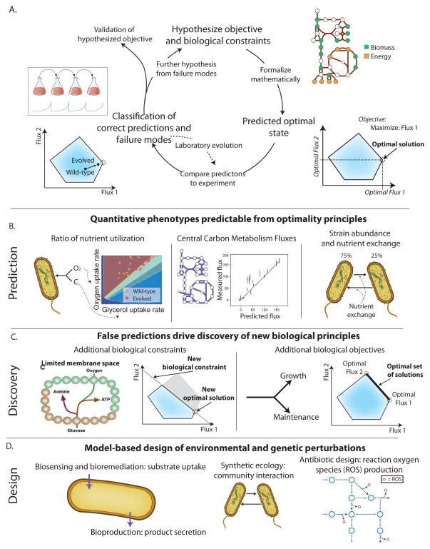
A. Quantitative phenotype prediction is an iterative workflow. First, hypothesized biological constraints and objectives are formulated mathematically, and computational optimization is used to determine optimal phenotypic states (see Section 2). The predicted phenotypic states can then be compared to experimental measurements to identify where predictions are consistent. When consistent, the hypothesized evolutionary objective and constraints are validated. When inconsistent, laboratory evolution can be used to gain further insight as to why the computed and measured states differ. Examples of validation of quantitative phenotypes are detailed in 4B and further hypotheses derived from incorrect predictions are detailed in 4C. B. The generic workflow in 4A has been successfully applied to several classes of phenotypes. i) Nutrient utilization ratios can be predicted by maximizing biomass flux (Edwards et al., 2001). ii) Central carbon metabolism fluxes can be predicted; for some organisms, much of the variability in flux can be attributed to biomass flux maximization (Schuetz et al., 2012). iii) The ratio of organism abundances and nutrient exchanges can be predicted for both natural and synthetic communities. Note that one important feature of quantitative phenotype predictions is that optimal flux solutions are often not unique. To address this, flux variability analysis (FVA) (Mahadevan and Schilling, 2003) can be used to identify the ranges of possible fluxes. It should be noted that non-uniqueness is not necessarily a handicap of COBRA as biological evolution can come up with alternate solutions (Fong et al., 2005). C. Inconsistencies with model predictions have led to the appreciation of new constraints and objectives underlying cellular phenotypes. i) Inconsistent predictions in by-product secretion have led to the hypothesis that membrane space limits membrane protein abundance and metabolic flux (Zhuang et al., 2011b). ii) The range of metabolic fluxes observed across different environments have led to the realization that fluxes can be understood as simultaneously satisfying multiple competing objectives, such as growth and cellular maintenance. Multi-objective optimization algorithms find solutions that maximize multiple competing objectives. D. Accurate prediction of quantitative phenotypes has led to prospective design of biological functions. A number of algorithms have been developed that predict genetic and/or environmental perturbations required to achieve a bioengineering objective. Relevant bioengineering objectives have included biosensing, bioremediation, bioproduction, the creation of synthetic ecologies, and the intracellular production of reaction oxygen species (ROS) to potentiate antibiotic effects.

Figure 5. Data integration and exploration of possible cellular phenotypes

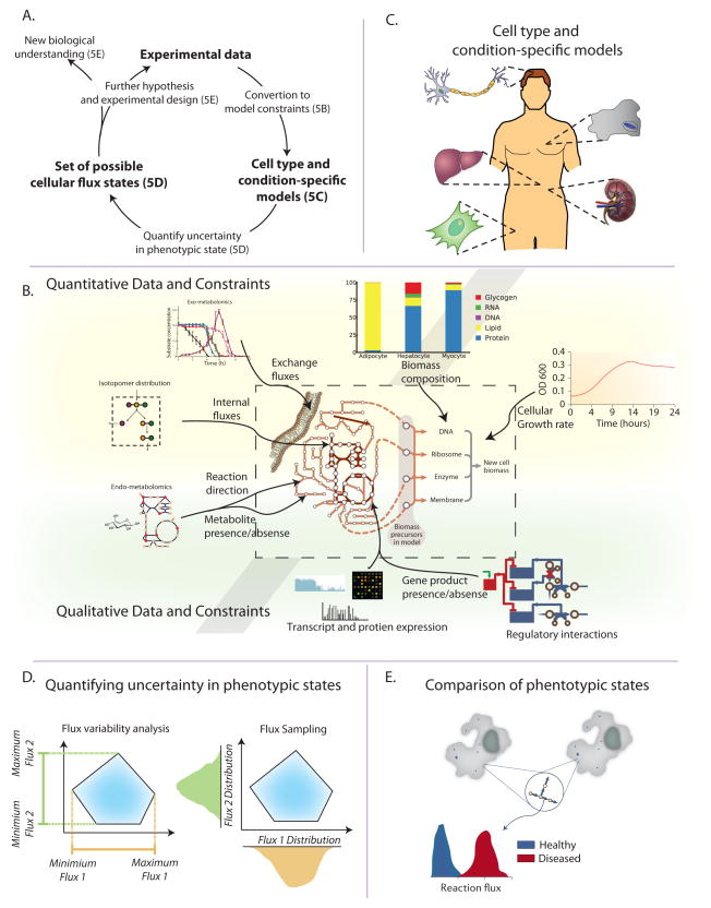
A. The general workflow for multi-omic data integration begins with the conversion of the experimental data into model constraints (see Figure 5B). This procedure results in cell-type (e.g. neuron, macrophage) and condition-specific (e.g. healthy vs. diseased) models that represent the metabolic capabilities of those specific cells (see Figure 5C). Several computational procedures can then be used to explore the metabolic capabilities and determine achievable phenotypes systematically (see Figure 5D). Evaluation of these phenotypic capabilities and comparison of different cells or environments leads to identification of their molecular differences (see Figure 5E). Additionally, if the original experimental data cannot precisely distinguish between certain metabolic states, additional targeted experiments can be designed and integrated as further constraints. B. Numerous data types can be integrated into metabolic models. Some directly affects model structure and variables (e.g. growth rate, biomass composition, exchange fluxes, internal fluxes and reaction directionality). Standard processing of these data types allows for integration into the model. Other data types affect metabolic fluxes more indirectly. As such, different computational methods exist for formulating the appropriate constraints (Table 1). C. Experimental data is integrated to construct cell-type and/or conditionspecific models. These models represent the metabolic capabilities in a certain state, and are then used for further inquiry (see Figures 5D,E). Specific algorithms for building cell-type specific models from gene expression data include MBA (Jerby et al., 2010) and GIMME (Becker and Palsson, 2008). D. After adding constraints to the model, computational procedures are used to assess the implication of the experimental data on metabolic fluxes. The two main methods for querying the consequences of the measured data on a cell’s phenotypes are flux variability analysis (FVA) and Markov-chain Monte-Carlo (MCMC) sampling. i) FVA determines the maximum and minimum values of all metabolic fluxes. ii) MCMC sampling randomly samples feasible metabolic flux vectors (usually resulting in tens to hundreds of thousands of flux vectors). These sampled flux vectors can then be used to derive the distribution of possible flux values for a given metabolic reaction. E. Often a comparative approach is employed in which experimental data from two conditions are used to generate two condition-specific models. Then, the achievable phenotypes of the two states are compared (e.g. though MCMC sampling, see Figure 5D).

Figure 6. Expansion of genome-scale models to encompass molecular biology

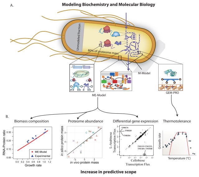
A. Metabolic models have been expanded to encompass the processes of proteome synthesis and localization as well as data on protein structures. Models including protein synthesis and localization are referred to as ME-Models, which stands for metabolism and gene expression. GEM-PRO refers to genome-scale models integrated with protein structures. For GEM-PRO, a combination of structural data directly references the GPRs in the metabolic reconstruction; structures can be obtained from experimental databases or homology modeling. The E. coli ME-Model mechanistically accounts for ~80% of the proteome mass in conditions of exponential growth and 100% of other major cell constituents (DNA, RNA, cell wall, lipids, etc). B. Addition of cellular processes vastly increases the predictive scope of models. ME-Models can predict biomass composition, abundances of protein across subsystems, and differential gene expression in certain environmental shifts (in addition to the predictions possible with M-Models); like FBA these were predicted by assuming growth maximization as an evolutionary objective, though the specific optimization algorithm differs due to the addition of coupling constraints. GEM-PRO has been used to predict the metabolic bottlenecks and growth defects of changes in temperature on protein stability and catalysis; protein stability is predicted with structural bioinformatics methods and then used to limit the catalyzed metabolic flux. The uses of these integrated models are just beginning to be explored.