Endogenous sequential cortical activity evoked by visual stimuli

Abstract

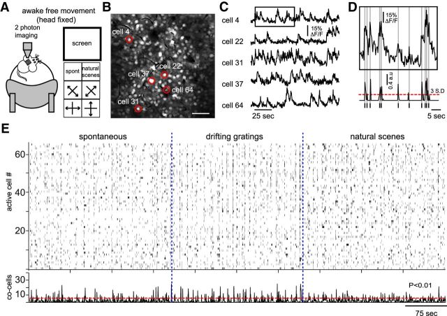
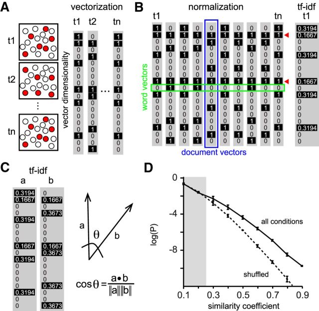
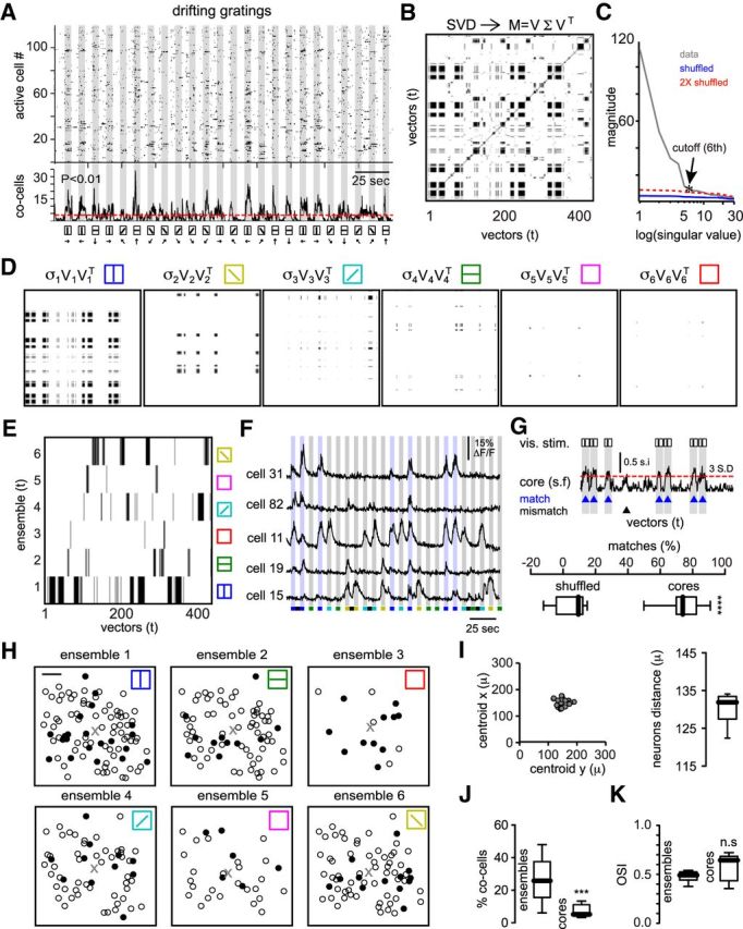
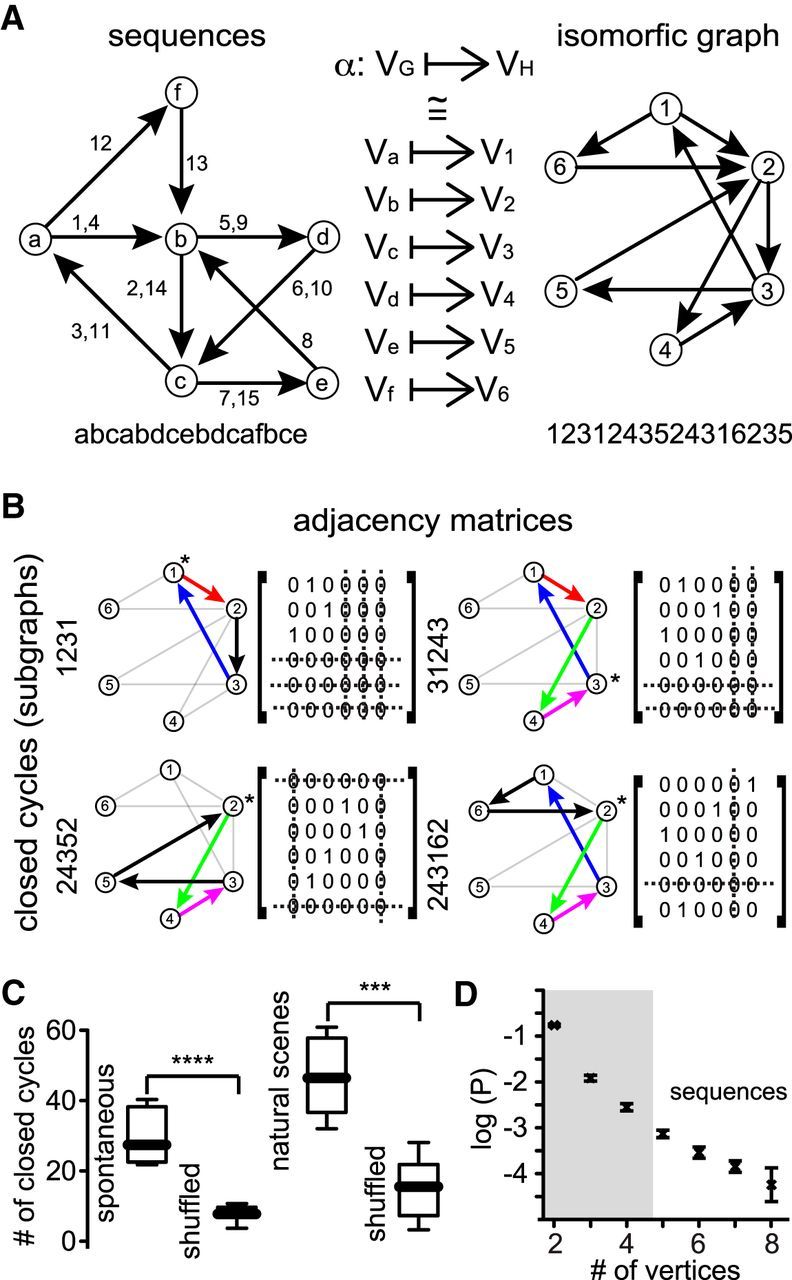
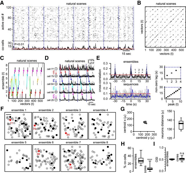
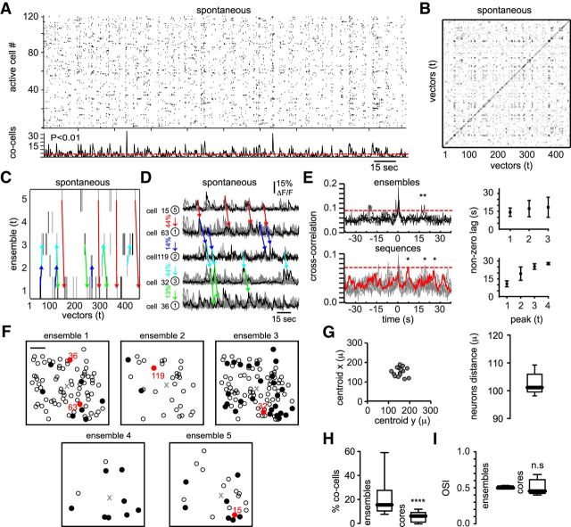
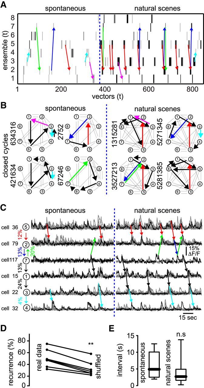
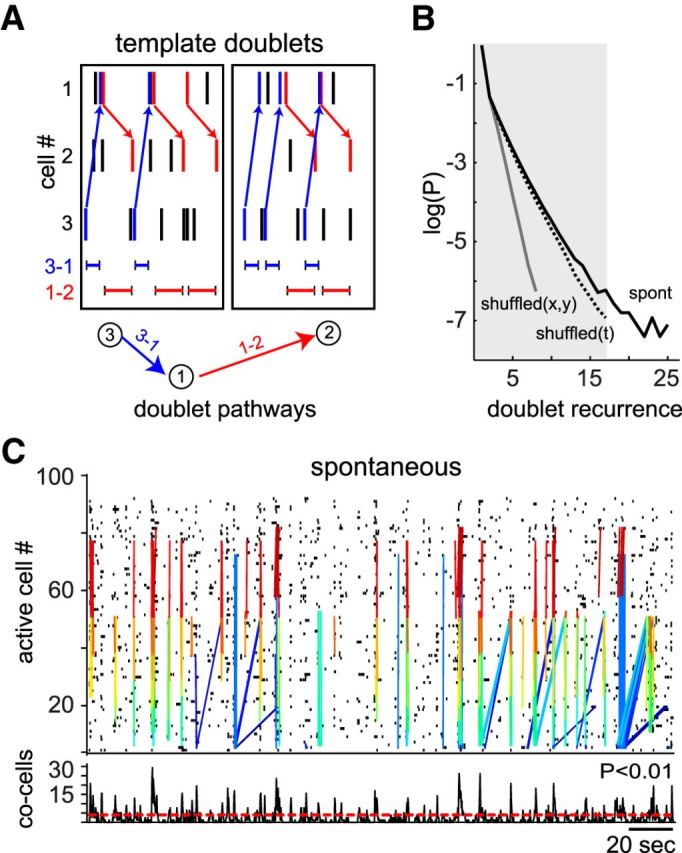
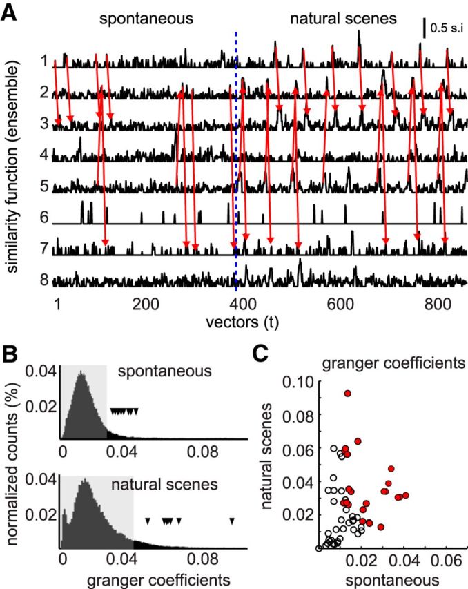
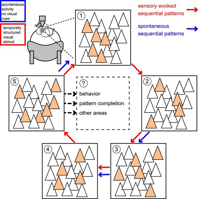
Although the functional properties of individual neurons in primary visual cortex have been studied intensely, little is known about how neuronal groups could encode changing visual stimuli using temporal activity patterns. To explore this, we used in vivo two-photon calcium imaging to record the activity of neuronal populations in primary visual cortex of awake mice in the presence and absence of visual stimulation. Multidimensional analysis of the network activity allowed us to identify neuronal ensembles defined as groups of cells firing in synchrony. These synchronous groups of neurons were themselves activated in sequential temporal patterns, which repeated at much higher proportions than chance and were triggered by specific visual stimuli such as natural visual scenes. Interestingly, sequential patterns were also present in recordings of spontaneous activity without any sensory stimulation and were accompanied by precise firing sequences at the single-cell level. Moreover, intrinsic dynamics could be used to predict the occurrence of future neuronal ensembles. Our data demonstrate that visual stimuli recruit similar sequential patterns to the ones observed spontaneously, consistent with the hypothesis that already existing Hebbian cell assemblies firing in predefined temporal sequences could be the microcircuit substrate that encodes visual percepts changing in time.

Keywords: graph theory; in vivo calcium imaging; multidimensional population vectors; neuronal ensembles; primary visual cortex; two-photon microscopy.

Figure 1.

Two-photon imaging of population activity in primary visual cortex of freely moving animals. A, Experimental setup. Mice are head fixed to the stage of a two-photon microscope on top of a foam ball floating in air that allows them to move freely. A monitor placed 15 cm contralateral to the craniotomy site displays different visual stimuli that are computer controlled and consist of drifting gratings of four orientations moving in two different directions, nonstimulus or natural scenes. For simplicity, orientation bars are represented by lines and not the actual patterns presented. B, Visual cortical neurons bulk loaded with Oregon green showing the average of 1000 consecutive frames. White dots indicate individual cells. Red circles indicate neurons shown in C. Scale bar, 50 μm. C, Calcium transients recorded from the cells shown in B. Cortical neurons have episodes of spontaneous activity. D, Spike detection of the calcium transients taken from the insert in C. Lines on bottom (spikes) indicate neuronal activity. Dashed line indicates a threshold >3 times the SD of noise. Spikes were used to construct binary arrays representing the activity of each neuron. E, Raster plot representing the overall activity of the network in different experimental conditions is shown at the top. Each row represents an active neuron. Temporal histogram of the spontaneous activity observed in cortical neurons is shown at the bottom. Dashed line indicates a threshold value used to select the synchrony peaks with a low probability (p < 0.01) of being random. Note the presence of spontaneous periods of synchronous activity without apparent periodicity.

Figure 2.

Representation of network activity as multidimensional arrays. A, Schematic representation of network activity vectorization. Each vector represents a group of neurons firing in synchrony at a given time point. Cells active at different times (t1, t2, tn) are highlighted in red (left). Each frame is represented as a binary vector of “n” dimensions. The dimensionality of the vectors is given by the total number of active cells in a specific field of view (80 ± 25 neurons; n = 7 mice). B, TF–IDF normalization was calculated to decrease the overall weight of neurons with high activity (red marks). C, Schematic representation of cosine similarity used to define repeated activity patterns. D, Probability distribution of similarity coefficients from all possible vector pairs between three different experimental conditions. Shaded area denotes not significant values (p > 0.05) for a range of similarity coefficients. For similarity coefficients >0.24, real data are significantly different from shuffled data.

Figure 3.

Neuronal ensembles define recurrent groups of neurons responding to specific visual stimuli. A, Raster plot of network activity responses to drifting gratings (top). Each row represents an active neuron. Gray stripes indicate the duration of the stimuli. Temporal histogram represents the number of coactive cells over time (middle). Dashed line indicates a threshold value used to select the synchrony peaks with low probability (p < 0.01) of being random events. Note that peaks of synchronous activity can be observed also in the absence of visual stimulation. Four different orientations and two directions were presented randomly (bottom). B, Binary matrix extracted from similarity map representing significant patterns of activity factorized by SVD. Black patterns indicate recurrent coactive cells at different moments. C, Magnitude of singular values used to determine the number of neuronal ensembles. Red line indicates 2× the magnitude of singular values from shuffled data. Cutoff value indicates the most representative number of neuronal ensembles corresponding to a significant change in slope of the magnitude of contiguous singular values. Networks of 80 ± 25 neurons stimulated with four drifting gratings can be defined by 6 ± 1 neuronal ensembles (n = 7 mice). D, First six factors of SVD that reproduce reliably the overall behavior of the network. Bars on top indicate orientations; empty squares represent recurrent neuronal ensembles appearing in the absence of visual stimuli. E, Neuronal ensembles sorted in time defined by the most representative factors of singular value decomposition. Each row represents a neuronal ensemble. Note that some neuronal ensembles occurred spontaneously in the absence of visual stimulation (empty squares). A neuronal ensemble represents a group of cells with synchronous, recurrent, and alternating activity. F, Calcium transients from five of the most representative cells that defined neuronal ensemble 1 (blue; 90 degrees orientation). Blue stripes represent visual stimuli with 90 degrees orientation. Some cells responded to only one orientation and others responded to multiple orientations. Colors on bottom depict different orientations. Note that neuronal ensembles entrained by drifting gratings represent neurons with synchronous and recurring activity imposed by visual stimuli. G, Similarity function of the most representative neurons (core) responding to 90 degrees orientation (top). A threshold of 3 times the SD of the noise indicates when a specific neuronal ensemble matches a given drifting grating (blue). The percentage of matches demonstrates that core ensembles can predict when a given visual stimuli was presented (bottom; p < 0.0001; Mann–Whitney test). H, Spatial maps of the neurons belonging to different neuronal ensembles. Black cells show the most representative neurons of each ensemble (core) that can reproduce the overall behavior of the network. Scale bar, 50 μm. I, Center of mass from different ensembles (left) and the mean distance between all of the neurons from each ensemble (right) demonstrate that ensembles are anatomically widespread. J, Percentage of coactive cells between ensembles and core ensembles (p = 0.0001; Mann–Whitney test). K, Orientation selectivity index from neurons belonging to ensembles or cores (p = 0.3095; Mann–Whitney test). Note that cells with broad tuning can be part of core ensembles.

Figure 4.

Identification of closed cycles of activity describing sequential activity patterns using graph theory. A, Cell assemblies described by Hebb. Each letter represents a group of neurons firing in synchrony. Arrows depict the transition between two neuronal ensembles. Numbers indicate the transition between different neuronal ensembles as a time function. Letters on bottom indicate the “sentence” describing all of the transitions. The graph depicting sequential patterns defined by Hebb can be transformed by graph theory in an isomorphic graph in which each vertex represents only one vertex of the original graph. Numbers on bottom indicate transitions between neuronal ensembles in function of time. B, Closed cycles of activity extracted from the isomorphic graph that depicts the transitions between neuronal ensembles. Each closed cycle is defined by a unique adjacency matrix. Note that some pathways can be part of different closed cycles. C, Total number of closed cycles that can be found during spontaneous (p < 0.0001; Mann–Whitney test) and visually evoked activity (p = 0.0007; Mann–Whitney test) in real and shuffled data. Note that exactly the same closed cycles that appeared in real data were never found in shuffled data. D, Probability distribution of finding a specific sequence in a closed cycle as a function of the number of vertices. Note that, for closed cycles with >4 vertices, the probability of finding a specific sequence is above chance levels (p < 0.05).

Figure 5.

Visual stimulation with natural scenes trigger sequential activity patterns. A, Raster plots representing the overall network activity evoked by 10 different natural scenes presented recurrently in exactly the same temporal order (blue dashed vertical lines delimit the duration of each sequence). B, Similarity map illustrating the visualization of recurrent sequential activity patterns. Note that stereotyped transitions between neuronal ensembles are represented by lines parallel to the main diagonal. C, Neuronal ensembles sorted in time representing stereotyped sequential activity patterns from the network activity reflecting the same series of scenes presented many times. Neuronal ensembles are locked in time to visual stimuli. D, Calcium transients of the most representative cells belonging to a specific neuronal ensemble. Numbers depict neuronal ensembles. Percentages indicate the conditional probability to go from one neuronal ensemble to another. Dotted lines delimit the beginning of the same sequence of natural scenes. Note that stereotyped sequential activity patterns can be observed at the single-cell level. E, Cross-correlation plots (left) of neurons belonging to the same neuronal ensemble (top) and neurons belonging to different neuronal ensembles firing in sequence (bottom). Each trace represents the average of all possible combinations of neurons. Red lines denote confidence levels. Significant cross-correlation peaks at nonzero time lags (right) demonstrate that ensemble responses are tied to the visual stimuli presented. Note that visual stimulation triggers recurrent sequential activity patterns. F, Spatial maps of the neurons belonging to each neuronal ensemble. Black cells indicate the most representative cells. Red neurons show the ones highlighted in D. Scale bar, 50 μm. G, Center of mass from different ensembles (left) and the mean distance between all of the neurons from each ensemble (right) demonstrate that ensembles are anatomically widespread. H, Percentage of coactive cells between ensembles and core ensembles (p < 0.0001; Mann–Whitney test). I, Orientation selectivity index from neurons belonging to ensembles or cores (p = 0.5054; Mann–Whitney test). Note that cells with broad tuning can be part of core ensembles.

Figure 6.

Sequential activity patterns are present in spontaneous activity. A, Raster plots representing the overall network activity in the absence of visual stimulation. B, Similarity map illustrating recurrent sequential activity patterns. Note repeated structures at different times. C, Neuronal ensembles sorted in time. Recurrent transitions between neuronal ensembles are denoted by arrows. D, Calcium transients of the most representative cells defining each neuronal ensemble. Each arrow defines a pathway between two neuronal ensembles. Note repetitive sequential patterns that appeared spontaneously without visual stimuli. Percentages indicate the conditional probability between two different neuronal ensembles. E, Cross-correlation plots (left) of neurons belonging to the same neuronal ensemble (top) and neurons belonging to different neuronal ensembles firing in sequence (bottom). Red color represents the transition between ensemble number 5 and ensemble number 1. Significant peaks at nonzero time lag (right) show that spontaneous ensembles (top) and sequences (bottom) can appear at different time intervals. F, Spatial maps of the neurons belonging to each neuronal ensemble. Black cells indicate the most representative cells. Red neurons show the ones highlighted in D. Scale bar, 50 μm. G, Center of mass from different ensembles (left) and the mean distance between all of the neurons from each ensemble (right) demonstrate that ensembles are anatomically widespread. H, Percentage of coactive cells between ensembles and core ensembles (p < 0.0001; Mann–Whitney test). I, Orientation selectivity index from neurons belonging to ensembles or cores (p = 0.6905; Mann–Whitney test). Note that cells with broad tuning can be part of core ensembles.

Figure 7.

Similarity between endogenous and evoked sequential activity patterns. A, Neuronal ensembles sorted in time representing spontaneous activity (left) can also be evoked by repetitive visual stimulation (right). Note the existence of stereotyped activity during natural stimuli conditions reflecting the same series of scenes presented many times. Note that sequential activity patterns elicited by natural stimuli were also present in spontaneous activity before exposure to visual stimuli. B, Graph theory techniques applied to the transitions between neuronal ensembles depicted sequential activity patterns (colored arrows) that appeared spontaneously (left) and in the presence of natural stimuli (right). Each colored arrow defines a pathway between two neuronal ensembles that is present in both conditions. C, Calcium transients of the most representative cells belonging to each neuronal ensemble in the absence (left) and the presence (right) of visual stimuli. Percentages indicate the conditional probability to go from one neuronal ensemble to another. Note that sequential patterns recruited by natural stimuli are also present in spontaneous activity. Visual stimulation triggers endogenous generated neuronal ensembles, indicating that sequential activity patterns recruited by sensory input are imprinted in the network. D, Total number of sequences that can be found in spontaneous activity that were recruited by visual stimulation compared with the number of sequences that can be found in shuffled data. Note that the recurrence between spontaneous and natural scenes is statistically significant compared with the shuffled condition (p = 0.0078; Wilcoxon matched-pairs signed-rank test). E, Interval of recurrent sequences in spontaneous activity compared with natural scenes is not significantly different (p = 0.1488; Mann–Whitney test).

Figure 8.

Precise firing patterns underlie sequential activity. A, Schematic representation of template doublets. A doublet is defined as a recurrent sequence between two cells with fixed time interval occurring above chance. Each color depicts a different doublet pathway repeated at distinct time points. B, Probability distribution of doublet recurrence used to determine doublets above chance levels. Doublets represent alternate pathways of activity. Note that doublet analysis is independent from neuronal ensemble identification. However, doublets and neuronal ensembles demonstrate temporally structured network activity in primary visual cortex. C, Raster plot of spontaneous activity from visual cortical neurons showing doublets. Each color denotes the same pair of neurons firing in sequence with a fixed time interval. Doublet elements appeared during spontaneous peaks of synchronous activity (bottom).

Figure 9.

Prediction of future neuronal ensembles. A, Similarity function across time for each neuronal ensemble during spontaneous and evoked activity. Note that the similarity index increases every time that a given ensemble is active. Red arrows indicate transitions between different ensembles. B, Granger causality analysis supports the predictive relationships between ensemble pairs. Granger causality coefficients (change in R²) between several neuronal ensemble pairs occur above chance levels (black triangles). Random coefficients were calculated between all ensemble pairs by independently shifting time courses within pairs 1000 times. Dashed areas denote 95% of the random distribution of all possible combinations between ensembles. C, Scatterplots of Granger coefficients showing that transitions between two neuronal ensembles appearing spontaneously can be entrained by natural stimuli. Significant ensemble pairs from B are filled circles.

Figure 10.

Diagram summarizing sequential activity patterns. Visual stimuli recruit preexistent sequential activity patterns. Each neuronal ensemble is defined by a group of cells firing in synchrony. Numbers indicate different neuronal ensembles (colored neurons denote active cells). The same groups of cells could define neuronal ensembles during spontaneous activity and visual stimulation. Arrows represent sequential transitions between different neuronal ensembles. Sequential activity patterns entrained by visual stimuli could drive behavioral outcomes, perform pattern completion, or transfer time information to other cortical areas. Red arrows denote sequential patterns recruited by visual stimulation; blue arrows indicate preexistent sequential patterns present in spontaneous activity. Sensory evoked activity can recruit preexistent temporal pathways found in spontaneous activity.

References

1. Abeles M. Corticonics. Cambridge: Cambridge University; 1991.
1. Abeles M, Bergman H, Margalit E, Vaadia E. Spatiotemporal firing patterns in the frontal cortex of behaving monkeys. J Neurophysiol. 1993;70:1629–1638. - PubMed
1. Abeles M, Hayon G, Lehmann D. Modeling compositionality by dynamic binding of synfire chains. J Comput Neurosci. 2004;17:179–201. doi: 10.1023/B:JCNS.0000037682.18051.5f. - DOI - PubMed
1. Ayzenshtat I, Meirovithz E, Edelman H, Werner-Reiss U, Bienenstock E, Abeles M, Slovin H. Precise spatiotemporal patterns among visual cortical areas and their relation to visual stimulus processing. J Neurosci. 2010;30:11232–11245. doi: 10.1523/JNEUROSCI.5177-09.2010. - DOI - PMC - PubMed
1. Baeg EH, Kim YB, Huh K, Mook-Jung I, Kim HT, Jung MW. Dynamics of population code for working memory in the prefrontal cortex. Neuron. 2003;40:177–188. doi: 10.1016/S0896-6273(03)00597-X. - DOI - PubMed
Publication types
LinkOut - more resources