A Unifying Model for Capture-Recapture and Distance Sampling Surveys of Wildlife Populations

Abstract

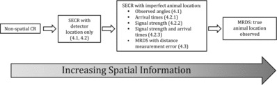
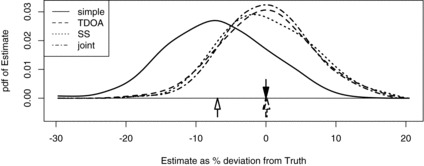
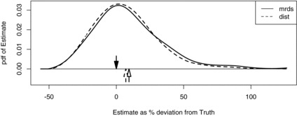
A fundamental problem in wildlife ecology and management is estimation of population size or density. The two dominant methods in this area are capture-recapture (CR) and distance sampling (DS), each with its own largely separate literature. We develop a class of models that synthesizes them. It accommodates a spectrum of models ranging from nonspatial CR models (with no information on animal locations) through to DS and mark-recapture distance sampling (MRDS) models, in which animal locations are observed without error. Between these lie spatially explicit capture-recapture (SECR) models that include only capture locations, and a variety of models with less location data than are typical of DS surveys but more than are normally used on SECR surveys. In addition to unifying CR and DS models, the class provides a means of improving inference from SECR models by adding supplementary location data, and a means of incorporating measurement error into DS and MRDS models. We illustrate their utility by comparing inference on acoustic surveys of gibbons and frogs using only capture locations, using estimated angles (gibbons) and combinations of received signal strength and time-of-arrival data (frogs), and on a visual MRDS survey of whales, comparing estimates with exact and estimated distances. Supplementary materials for this article are available online.

Keywords: Abundance estimation; Acoustic survey; Closed population; Measurement error; Visual survey.

Figure 1. A continuum of increasingly spatially resolved capture–recapture models. Numbers in brackets correspond to subsections of the article.

Figure 2. Example location estimates, given capture, of two different gibbons. Detectors are crosses; circled detectors are those that detected the gibbon call. Arrows show estimated angles to detections. Dotted lines are the contours of the estimated probability of the group being contained within the contour, given only the spatial capture history data Ω. Dashed lines are estimated contours, given only observed angles to detections. Solid lines are estimated contours, given capture history and angles.

Figure 3. Smoothed simulated sampling distributions of estimated gibbon call density when only spatial capture history is used in estimation (“simple”) and when capture history and observed angles are used (“angle”). The down arrow marks true (simulated) density, the horizontal axis is percentage deviation from true density, and the up arrows are the means of the sampling distributions.

Figure 4. Estimated location contours given capture history and SS (left) and capture history and TDOA (right), of a click. Detectors are crosses; circled detectors are those that detected the frog click. Dotted lines are the contours of the probability density of frog location given only spatial capture history data Ω. Dashed lines in the right plot are contours given only TDOA. Solid lines are contours of location given capture history and SS (left) or capture history and TDOA (right).

Figure 5. Smoothed simulated sampling distributions of estimated frog click density using only spatial capture history (“simple”), using capture history and time of arrival (“TDOA”), using capture history and signal strength (“SS”), and using capture history, time of arrival and signal strength (“joint”). The down arrow marks true density, the horizontal axis is percentage deviation from true density, and the up arrows are the means of the sampling distributions, expressed as percentage deviation from truth (some are almost coincident).

Figure 6. Estimated location contours (dotted) given capture history and recorded location (solid) of a whale detected by one of the two detectors. Contours are such that 100α% of the density falls between the two contours marked α. The left plot shows locations in perpendicular and forward distance space, the right curve shows it in radial distance space. Detectors are crosses.

Figure 7. Smoothed simulated sampling distributions of estimated whale cue density when capture history and exact distances are observed (“mrds”) and when capture history and estimated distances are used (“dist”). The down arrow marks true density, the horizontal axis is percentage deviation from true density, and the up arrows are the means of the sampling distributions.

References

1. Bonner S. Response to: A New Method for Estimating Animal Abundance With Two Sources of Data in Capture-Recapture Studies. Methods in Ecology and Evolution. 2013;4:585–588.
1. Borchers D.L. Line Transect Abundance Estimation With Uncertain Detection on the Trackline. 1996 PhD Thesis, University of Cape Town, Cape Town.
1. Borchers D.L. Buckland S.T. Zucchini W. Estimating Animal Abundance: Closed Populations. London: Springer; 2002.
1. Borchers D.L. Efford M.G. Spatially Explicit Maximum Likelihood Methods for Capture-Recapture Studies. Biometrics. 2008;64:377–385. - PubMed
1. Borchers D.L. Laake J.L. Southwell C. Paxton C. G.M. Accommodating Unmodelled Heterogeneity in Double-Observer Distance Sampling Surveys. Biometrics. 2006;62:372–378. - PubMed