Review
. 2014 Nov 19;1(3):140216.
doi: 10.1098/rsos.140216. eCollection 2014 Nov.

An investigation of the false discovery rate and the misinterpretation of p-values

Affiliations
Review

An investigation of the false discovery rate and the misinterpretation of p-values

David Colquhoun. R Soc Open Sci. .

Abstract

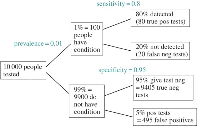
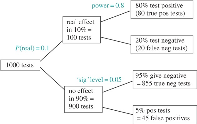
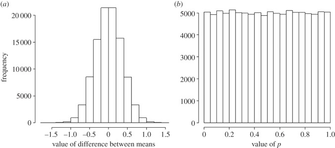
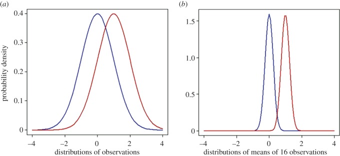
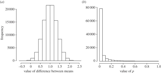
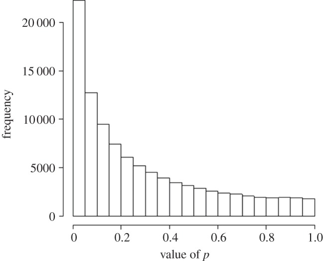
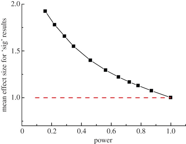
If you use p=0.05 to suggest that you have made a discovery, you will be wrong at least 30% of the time. If, as is often the case, experiments are underpowered, you will be wrong most of the time. This conclusion is demonstrated from several points of view. First, tree diagrams which show the close analogy with the screening test problem. Similar conclusions are drawn by repeated simulations of t-tests. These mimic what is done in real life, which makes the results more persuasive. The simulation method is used also to evaluate the extent to which effect sizes are over-estimated, especially in underpowered experiments. A script is supplied to allow the reader to do simulations themselves, with numbers appropriate for their own work. It is concluded that if you wish to keep your false discovery rate below 5%, you need to use a three-sigma rule, or to insist on p≤0.001. And never use the word 'significant'.

Keywords: false discovery rate; reproducibility; significance tests; statistics.


Figures

Figure 1.
Figure 1.
Tree diagram to illustrate the false discovery rate in screening tests. This example is for a prevalence of 1%, specificity 95% and sensitivity 80%. Out of 10 000 people screened, 495+80=575 give positive tests. Of these, 495 are false positives so the false discovery rate is 86%.
Figure 2.
Figure 2.
Tree diagram to illustrate the false discovery rate in significance tests. This example considers 1000 tests, in which the prevalence of real effects is 10%. The lower limb shows that with the conventional significance level, p=0.05, there will be 45 false positives. The upper limb shows that there will be 80 true positive tests. The false discovery rate is therefore 45/(45+80)=36%, far bigger than 5%.
Figure 3.
Figure 3.
Results of 100 000 simulated t-tests, when the null hypothesis is true. The test looks at the difference between the means of two groups of observations which have identical true means, and a standard deviation of 1. (a) The distribution of the 100 000 ‘observed’ differences between means (it is centred on zero and has a standard deviation of 0.354). (b) The distribution of the 100 000 p-values. As expected, 5% of the tests give (false) positives (p≤0.05), but the distribution is flat (uniform).
Figure 4.
Figure 4.
The case where the null hypothesis is not true. Simulated t-tests are based on samples from the postulated true distributions shown: blue, control group; red, treatment group. The observations are supposed to be normally distributed with means that differ by 1 s.d., as shown in (a). The distributions of the means of 16 observations are shown in (b).
Figure 5.
Figure 5.
Results of 100 000 simulated t-tests in the case where the null hypothesis is not true, but as shown in figure 4. (a) The distribution of the 100 000 ‘observed’ values for the differences between means of 16 observations. It has a mean of 1, and a standard deviation of 0.354. (b) The distribution of the 100 000 p-values: 78% of them are equal to or less than 0.05 (as expected from the power of the tests).
Figure 6.
Figure 6.
Distribution of 100 000 p-values from tests like those in figure 5, but with only four observations in each group, rather than 16. The calculated power of the tests is only 0.22 in this case, and it is found, as expected, that 22% are p≤0.05.
Figure 7.
Figure 7.
The average difference between means for all tests that came out with p≤0.05. Each point was found from 100 000 simulated t-tests, with data as in figure 4. The power of the tests was varied by changing the number, n, of ‘observations’ that were averaged for each mean. This varied from n=3 (power=0.157) for the leftmost point, to n=50 (power=0.9986) for the rightmost point. Intermediate points were calculated with n=4, 5, 6, 8, 10, 12, 14, 16 and 20.

References

    1. Sellke T, Bayarri MJ, Berger JO. 2001. Calibration of p values for testing precise null hypotheses. Am. Stat. 55, 62–71. (doi:10.1198/000313001300339950) - DOI
    1. Ioannidis JP. 2005. Why most published research findings are false. PLoS Med. 2, e124 (doi:10.1371/journal.pmed.0020124) - DOI - PMC - PubMed
    1. Colquhoun D. Lectures on biostatistics. (http://www.dcscience.net/Lectures_on_biostatistics-ocr4.pdf)
    1. Scharre DW, Chang SI, Nagaraja HN, Yager-Schweller J, Murden RA. 2014. Community cognitive screening using the self-administered gerocognitive examination (SAGE). J. Neuropsychiatry Clin. Neurosci. 26, 369–375. (doi:10.1176/appi.neuropsych.13060145) - DOI - PubMed
    1. McCartney M. 2013. Would doctors routinely asking older patients about their memory improve dementia outcomes?: No. Br. Med. J. 346, 1745 (doi:10.1136/bmj.f1745) - DOI - PubMed