. 2015 Jul;18(7):1025-33.
doi: 10.1038/nn.4042. Epub 2015 Jun 15.

A neural network that finds a naturalistic solution for the production of muscle activity

Affiliations

A neural network that finds a naturalistic solution for the production of muscle activity

David Sussillo et al. Nat Neurosci. 2015 Jul.

Abstract

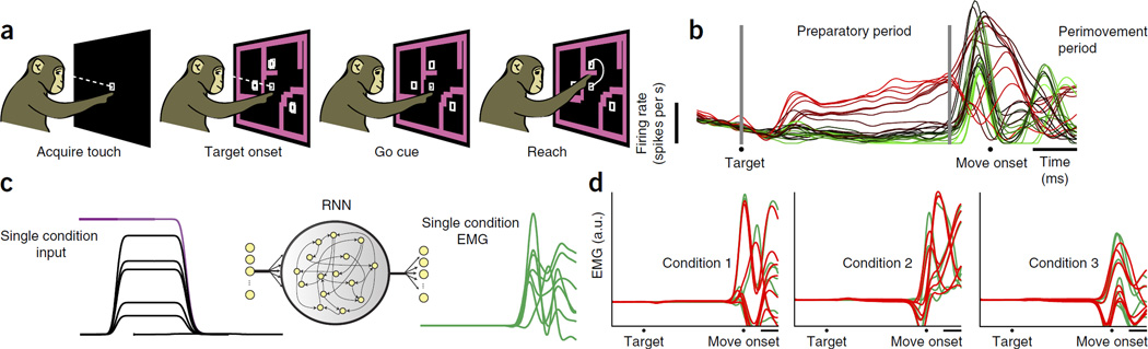
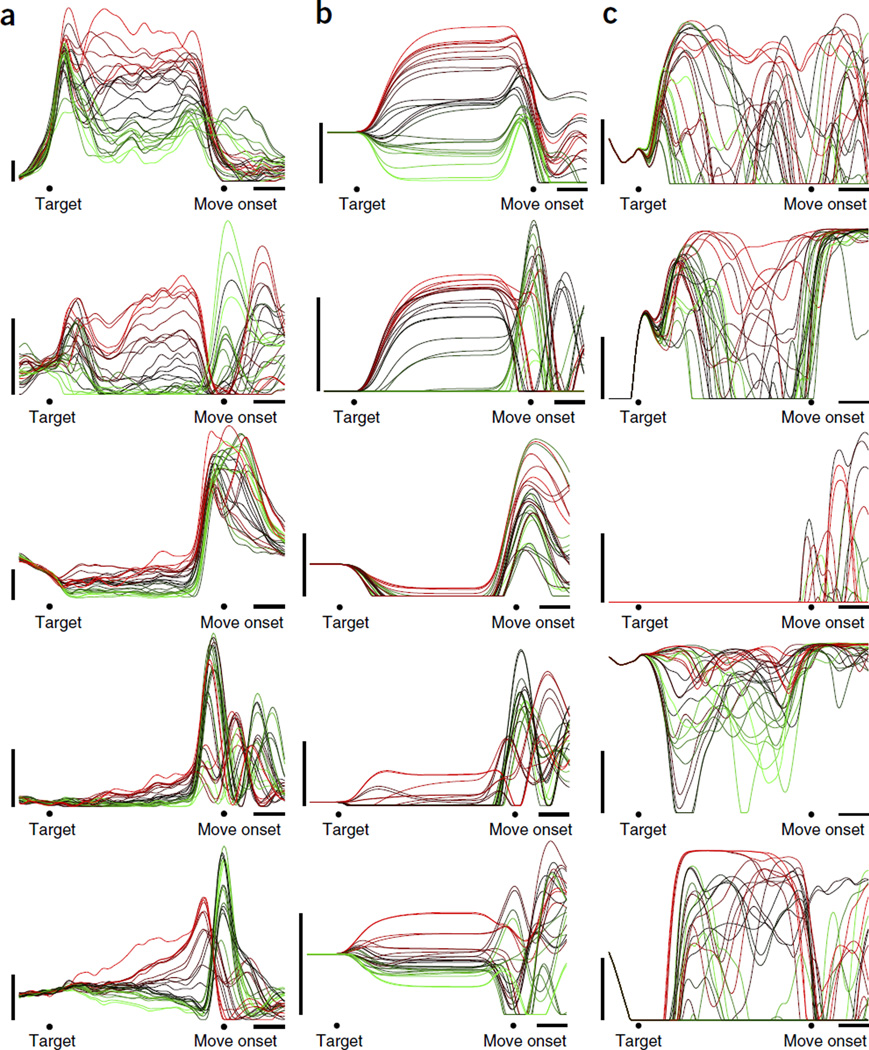
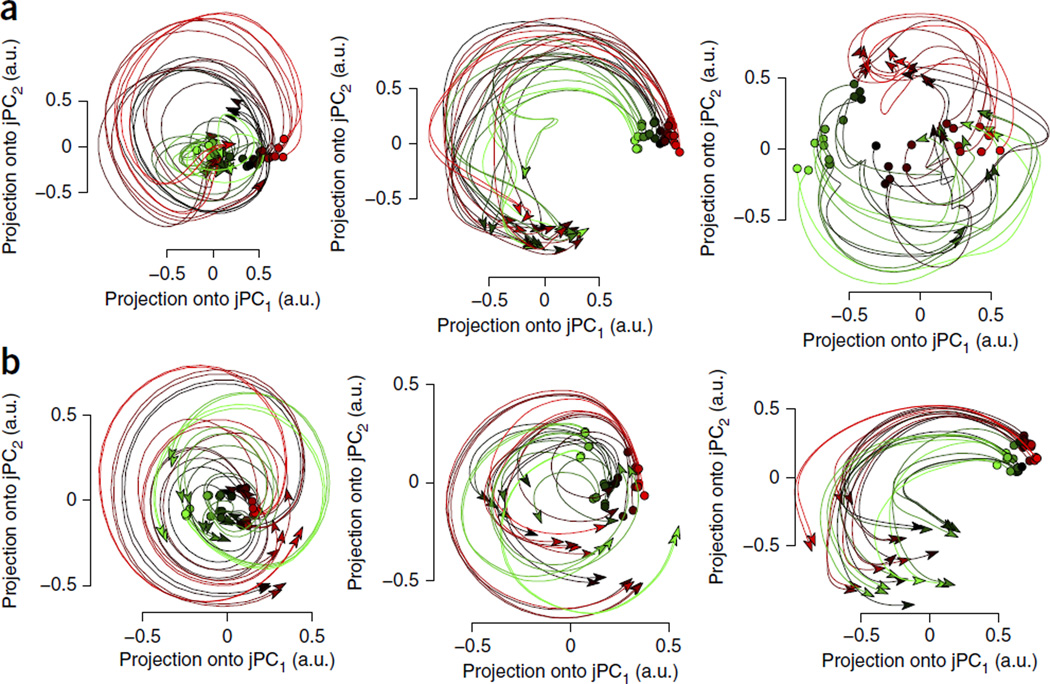
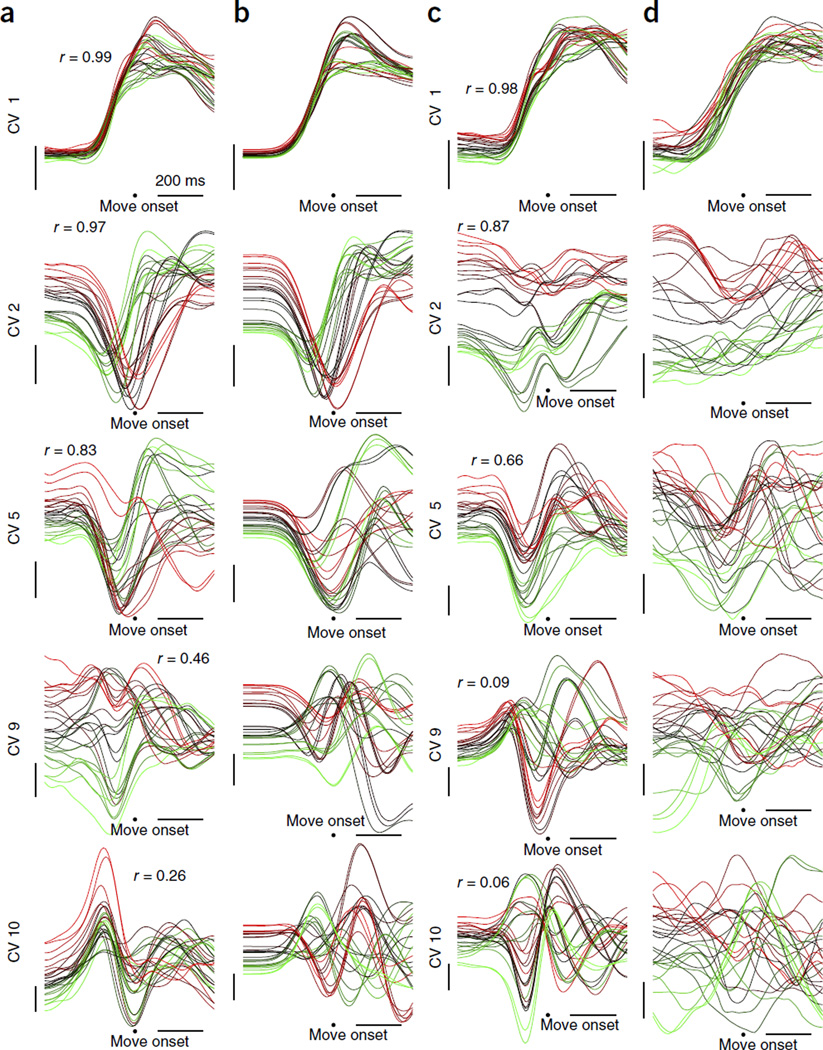
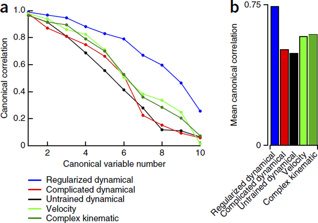
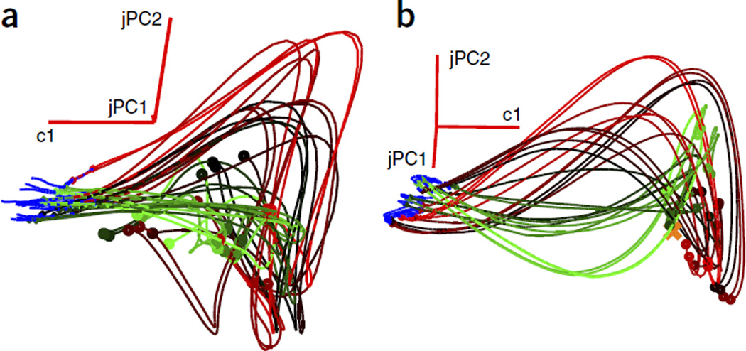
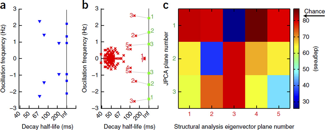
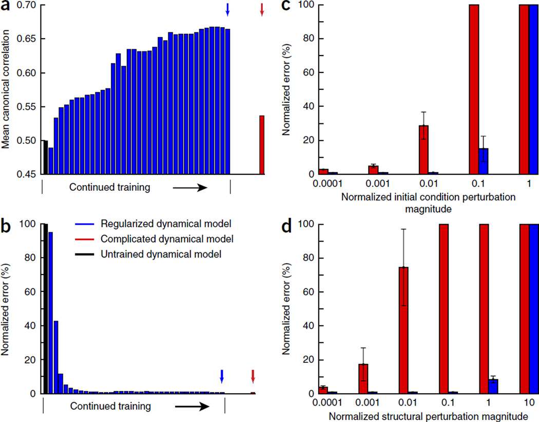
It remains an open question how neural responses in motor cortex relate to movement. We explored the hypothesis that motor cortex reflects dynamics appropriate for generating temporally patterned outgoing commands. To formalize this hypothesis, we trained recurrent neural networks to reproduce the muscle activity of reaching monkeys. Models had to infer dynamics that could transform simple inputs into temporally and spatially complex patterns of muscle activity. Analysis of trained models revealed that the natural dynamical solution was a low-dimensional oscillator that generated the necessary multiphasic commands. This solution closely resembled, at both the single-neuron and population levels, what was observed in neural recordings from the same monkeys. Notably, data and simulations agreed only when models were optimized to find simple solutions. An appealing interpretation is that the empirically observed dynamics of motor cortex may reflect a simple solution to the problem of generating temporally patterned descending commands.


Figures

Figure 1
Figure 1
Monkey task and network task definition. (a) Monkeys performed a delayed reach maze task. After fixating and touching a central point, the target and maze turned on. Some conditions included distractor targets. During the preparatory period, the monkeys had to determine which target was reachable and prepare a reach that avoided any intervening barriers. A go cue prompted the monkey to execute the reach. We employed 27 conditions, each consisting of a particular configuration of target and barriers. The resulting reaches included a variety of straight and curved paths. (b) Example PSTH for a single neuron. Each trace plots the mean across-trial firing rate for one condition (27 total). Traces are colored green to red based on the level of preparatory activity. The first gray line shows the timing of target onset, that is the beginning of the preparatory period. The second gray line shows the end of the preparatory period. Vertical and horizontal scale bars indicate 20 spikes per s and 200 ms. (c) Networks were optimized to generate EMG. Network inputs consisted of a condition-independent hold cue (purple) and a six-dimensional condition-specific input (black), which specified the condition for which the network should generate EMG. This example shows the levels of those six inputs for condition 1. From these inputs the RNN generated the multi-dimensional EMG: green traces plot the recorded EMG from seven muscles for condition 1. To ensure the model fit signal and not noise, we filtered EMG signals and removed the (very minimal) noise during the baseline (Online Methods). (d) Three example conditions showing the multiple muscle target EMG (green, one trace per muscle) and the corresponding trained outputs of the regularized model for monkey J (red). Normalized error between the empirical EMG and the model output was 7%. Horizontal scale bars indicate 200 ms.
Figure 2
Figure 2
Example PSTHs from monkey J and the regularized and complicated models for monkey J. (a) Example PSTHs from five neurons for monkey J (data are presented as in Fig. 1b). Examples were chosen to illustrate the range of responses, including neurons with strong preparatory activity (first two rows), neurons with a broad rise in activation during the movement period (middle row) and neurons with oscillatory activity during the movement period (bottom two rows). Vertical and horizontal scale bars indicate 20 spikes per s and 200 ms. (b) Example PSTHs chosen from the regularized model for monkey J. Examples were chosen to both highlight the similarities between neural and model responses and to be representative of the patterns exhibited by the model units. (c) Example PSTHs from five units from the complicated model for monkey J. The PSTHs of the complicated models rarely bore a strong resemblance to those of the neural data.
Figure 3
Figure 3
jPCA projections of the population responses. (a) jPCA projections for the neural data recorded from monkey J. Each trace shows the evolution of the neural state over 500 ms. Traces start −180 ms before movement onset, at the moment when the relatively stable preparatory state (circles) transitioned to the movement period trajectory. For visualization purposes, traces are colored on the basis of the preparatory-state projection onto jPC1 (a.u., arbitrary units). The three projections correspond to the largest magnitude complex eigenvalue pairs of the matrix Mskew, found when fitting the data with x˙=Mskewx (Online Methods). These eigenvalues correspond to frequencies of 2.1, 1.3 and 0.9 Hz (left to right) with a quality of fit (R2) for the optimal purely oscillatory linear system of 0.60. (b) jPCA projections for the regularized model of monkey J. Data are presented as in a. Frequencies are 2.4, 1.6 and 0.9 Hz. The linear system, x˙=Mskewx, had a quality of fit (R2) of 0.61.
Figure 4
Figure 4
Canonical correlations analysis for monkey J. (a,b) CCA projections (canonical variables) of the neural population response (a) and the regularized model for monkey J (b). These projections involve the directions in state-space that maximally correlate the neural data with the model data, resulting in a series of maximally to minimally correlated variables. Each row shows one of the canonical variables (CVs) 1, 2, 5, 9 and 10, highlighting the most and least similar projections. The correlation r is also shown. Traces are colored on the basis of the value of the projection at the beginning of the trace. The vertical scale bars indicate 1 arbitrary unit and the horizontal scale bars represent 200 ms. (c,d) Canonical variables of the neural population response (c) and the complicated model for monkey J (d) (data are presented as in a and b).
Figure 5
Figure 5
Comparison of simulated and neural population responses. (a) Summary of canonical correlations. CCA analysis provides a spectrum of correlation coefficients that can be used to directly compare one multidimensional data set to another. The canonical coefficients are shown for the various models, each compared with the neural data (blue indicates regularized dynamical model, also shown in Figure 4; red indicates complicated dynamical model, black indicates untrained complicated dynamical model with inputs, green indicates velocity model, dark green indicates complicated kinematic model). (b) The average of the canonical correlations (average of lines in a) between the models and the data. The average canonical correlation provides a single number for each model that quantifies how closely the model population response matches the recorded population response.
Figure 6
Figure 6
Monkey J and regularized model state-space visualizations. (a) Three-dimensional visualization of the neural data during the movement period for monkey J. The projection is comprised of the first jPC plane (Fig. 3a, left panel) and an additional dimension that captures variance from the cross-condition mean. Each trace is color-coded to show one of the 27 reach conditions. For all conditions, the trajectory during the preparatory period is colored blue. Time shown is 400 ms before to 220 ms after movement onset. Note that the jPC1 axis is projecting into the page. (b) Analogous three-dimensional visualization of the regularized model for monkey J (data are presented as in a). In addition, the single, condition-independent fixed point of the model, which organizes the dynamics of movement generation, is shown with an orange x. Time shown is 1,000 ms before to 220 ms after movement onset.
Figure 7
Figure 7
Frequency analysis of neural data and regularized model for monkey J. (a) Eigenvalue analysis of the neural data. Shown on the line of stability (Inf, neither decaying nor growing) are the purely imaginary eigenvalues associated with the jPCA analysis of the neural data in Figure 3a (blue squares). Also shown are the top eigenvalues of an unconstrained linear fit to the neural data (blue triangles). (b) The complex eigenvalue spectrum of the linearized system around the fixed point in the regularized model for monkey J (red x marks) based on a structural analysis of the weight matrix. Highlighted with red numbers are those modes of the linearized system that have a slow decay. Shown along the line of stability are the purely imaginary eigenvalues associated with the jPCA analysis of the regularized model data (green squares). Gray lines show the connection between the jPCA analysis and the structural analysis, as given by subspace angle analysis of eigenvectors in c. (c) Subspace angle analysis for the model, comparing the jPC planes (b, green squares) with the eigenvectors of the linearized system around the fixed point (b, red x marks). On the horizontal axis are listed the five slowest decaying oscillatory modes of the linearized system (corresponding to the red numbered modes in b). On the vertical axis are listed the three oscillatory planes found by jPCA (corresponding to the green numbered modes in b). Color indicates the minimum subspace angle (the minimum angle between the corresponding planes). For comparison, the minimum subspace angle between two randomly chosen planes in a N = 300 D space is 84 ±2 degrees (mean and s.d., black arrow labeled chance). Thus, a minimum subspace angle of 30–40 degrees indicates highly overlapping subspaces. In the present case, jPC plane 1 overlapped heavily with mode 3 (the highest frequency), jPC plane 2 overlapped heavily with oscillatory mode 2 (the second highest frequency) and jPC plane 3 overlapped more modestly with oscillatory mode 5 (the third highest frequency).
Figure 8
Figure 8
Regularization affects similarity to data and model robustness. (a) Average canonical correlation, as training progresses, between the regularized model and the neural data from monkey J. To provide a baseline, the black bar shows the mean canonical correlation between the untrained model with correct inputs and the neural data (0.50). As training with regularization progresses (blue), the model becomes more and more similar to the neural data, ending with a mean canonical correlation of 0.67 for this model (blue arrow). When trained to generate EMG without any regularization, the model has a mean canonical correlation with the data of 0.53 (red arrow). Black shows the canonical correlation of the untrained model with the data from monkey J. (b) The normalized error of the network output for the regularized model. Error decreased very quickly, even while the mean canonical correlation (a) continued to increase over a much longer period of training. The final error for the regularized model was comparable to the final training error for the complicated model (red). (c) Perturbation test of the initial conditions for the regularized and complicated models analyzed in a (blue and red arrows, respectively). The inputs were randomly perturbed according to a normalized percentage of the input strength (as given on horizontal axis). The network was then run and the mean normalized EMG error of the outputs (vertical axis) was averaged across 50 repetitions of this procedure. Error bars show s.d. The vertical axis is truncated at 100% error. (d) A structural perturbation test of the recurrent connectivity matrix in equation (1) for the regularized and complicated models analyzed in a (blue and red arrows, respectively). The connectivity matrix was randomly perturbed 50 times according to a normalized percentage of the mean absolute connection strength (as given on horizontal axis). The perturbed network was then run and the mean normalized EMG error of the outputs was averaged (vertical axis). Error bars show s.d. The vertical axis is truncated at 100% error.

References

    1. Evarts EV. Relation of pyramidal tract activity to force exerted during voluntary movement. J. Neurophysiol. 1968;31:14–27. - PubMed
    1. Mussa-Ivaldi FA. Do neurons in the motor cortex encode movement direction? An alternative hypothesis. Neurosci. Lett. 1988;91:106–111. - PubMed
    1. Sanger TD. Theoretical considerations for the analysis of population coding in motor cortex. Neural Comput. 1994;6:29–37.
    1. Todorov E. Direct cortical control of muscle activation in voluntary arm movements: a model. Nat. Neurosci. 2000;3:391–398. - PubMed
    1. Hatsopoulos NG. Encoding in the motor cortex: was evarts right after all? Focus on ‘motor cortex neural correlates of output kinematics and kinetics during isometric-force and arm-reaching tasks’. J. Neurophysiol. 2005;94:2261–2262. - PubMed

Publication types

LinkOut - more resources