ROCKETSHIP: a flexible and modular software tool for the planning, processing and analysis of dynamic MRI studies

Abstract

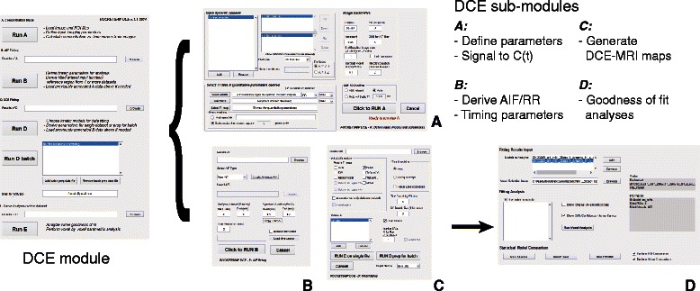
Background: Dynamic contrast-enhanced magnetic resonance imaging (DCE-MRI) is a promising technique to characterize pathology and evaluate treatment response. However, analysis of DCE-MRI data is complex and benefits from concurrent analysis of multiple kinetic models and parameters. Few software tools are currently available that specifically focuses on DCE-MRI analysis with multiple kinetic models. Here, we developed ROCKETSHIP, an open-source, flexible and modular software for DCE-MRI analysis. ROCKETSHIP incorporates analyses with multiple kinetic models, including data-driven nested model analysis.

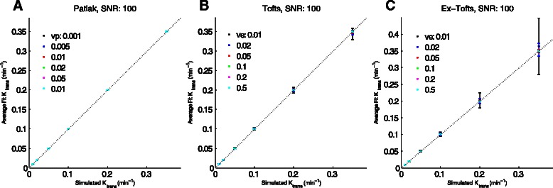
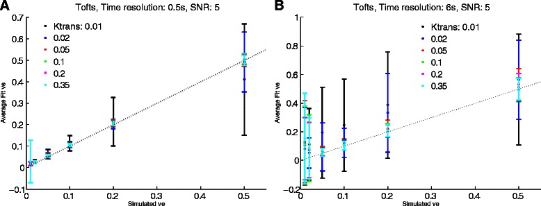
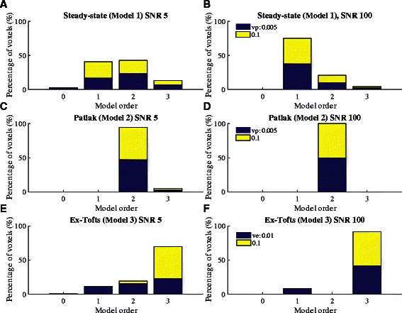
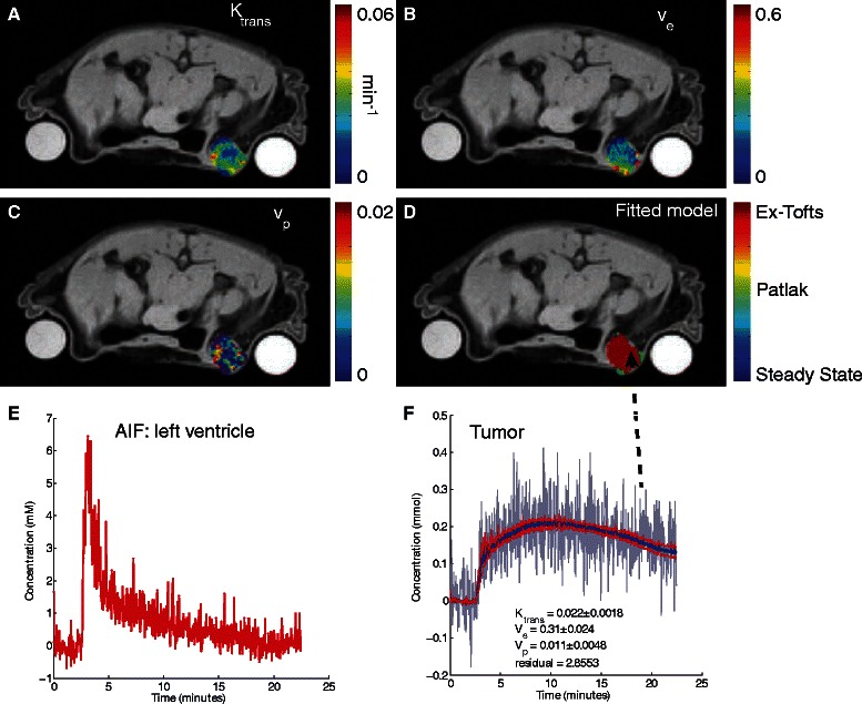
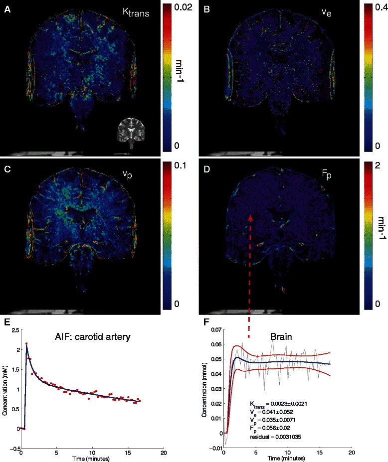
Results: ROCKETSHIP was implemented using the MATLAB programming language. Robustness of the software to provide reliable fits using multiple kinetic models is demonstrated using simulated data. Simulations also demonstrate the utility of the data-driven nested model analysis. Applicability of ROCKETSHIP for both preclinical and clinical studies is shown using DCE-MRI studies of the human brain and a murine tumor model.

Conclusion: A DCE-MRI software suite was implemented and tested using simulations. Its applicability to both preclinical and clinical datasets is shown. ROCKETSHIP was designed to be easily accessible for the beginner, but flexible enough for changes or additions to be made by the advanced user as well. The availability of a flexible analysis tool will aid future studies using DCE-MRI. A public release of ROCKETSHIP is available at https://github.com/petmri/ROCKETSHIP .

Fig. 1

Design outline of ROCKETSHIP. The software suite consists of a fitting module to generate T1, T2/T2* and ADC maps, and DCE-MRI module with sub-modules for each stage of DCE-MRI data processing and analysis

Fig. 2

DCE-MRI processing module GUI. GUI modules reflect the schematic outlined in Fig. 2. The “root” DCE module is shown on the left, which launches each sub-module in the pipeline. a defines the sub-module that converts raw image data to concentration time curves. The data are passed to the next sub-module, which allows temporal truncation of the dynamic data and fitting or importing of the AIF (b). DCE-MRI maps are derived using the next sub-module (c). Models can be generated in real time, or the user input can be saved as a data structure job to be run in batch later. Options are provided to perform voxel-by-voxel fits as well as defined ROIs. Raw data curves can be fitted as is, or after being passed through a time smoothing filter. Finally, goodness-of-fit analysis of the fits can be performed with the final sub-module (d)

Fig. 3

K_trans fitting of simulated data. Simulated data with time resolution of 0.5 s and SNR = 100 were fitted using the same model used to generate the simulation with ROCKETSHIP using default settings for the Patlak method (a), Tofts (b) and Extended Tofts models (c). K_trans simulated vs. fitted were plotted as a function of v_e and v_p. Dashed line is unity. Error bars denote standard deviation. Given the similar fits, points for different v_e and v_p may overlap. Concordance correlation coefficients for these (and other model fits) are shown in Tables 3, 4 and 5

Fig. 4

v_e fitting at different time resolutions. Simulated data using the Tofts model were generated at SNR = 5 and at time resolutions of 0.5 s (a) and 6 s (b). Simulated vs. fitted v_e were plotted as a function of K_trans. Dashed line is unity. Error bars represent standard deviation. As expected, lower time resolution results in a high standard deviation of the curve fits. Given the similar fits, points for different K_trans may overlap. Concordance correlation coefficients for these (and other model fits) are shown in Tables 3, 4 and 5

Fig. 5

Nested model selection from simulated data. a and b show fitting for steady-state model simulated data. c and d show the fitting for Patlak simulated data. All the generated curves at SNR = 100 converged to the correct model. At lower SNR, some of the curves incorrectly converged to Model 3 (extended Tofts). e and f show fitting on extended Tofts simulated data. Again, the majority of the curves converged to the correct model. The percentage of voxels attributed to each model by the nest model algorithm is shown in Table 6

Fig. 6

Nested model fitting of DCE-MRI data on a murine breast cancer tumor model. Parameters for K_trans (a), v_e (b), and v_p (c) are shown. As shown in d, the majority of the voxels fitted best to the extended Tofts model, with some edge voxels fitting to the Patlak method. e shows the AIF used for the fit (taken from the left ventricle). f shows a sample time curve from the edge of the tumor (denoted by arrow) with corresponding fit (blue denotes the fit, red lines denote the 95 % prediction bounds for the fitted curve). Rod phantoms on either side of the mouse were present to allow for signal drift correction (not used in this case)

Fig. 7

2CXM fitting of a normal human brain. Parameters for K_trans (a), v_e (b), v_p (c) and F_p (d) are shown. e shows the AIF used (taken from internal carotid artery). The AIF was fitted with a bi-exponential curve (blue) prior to tissue fitting. f shows a sample time curve from the brain parenchyma (denoted by arrow) with corresponding fit (blue denotes the fit, red lines denote the 95 % prediction bounds for the fitted curve). Fold over artifact is seen on the lateral brain edges due to truncation by the field of view bounding box

References

1. Parker GJ, Padhani AR. T1‐W DCE‐MRI: T1‐Weighted Dynamic Contrast‐Enhanced MRI. 2004. pp. 341–64.
1. Cuenod C, Fournier L, Balvay D, Guinebretiere J-M. Tumor angiogenesis: pathophysiology and implications for contrast-enhanced MRI and CT assessment. Abdom Imaging. 2006;31(2):188–93. doi: 10.1007/s00261-005-0386-5. - DOI - PubMed
1. Hylton N. Dynamic contrast-enhanced magnetic resonance imaging as an imaging biomarker. J Clin Oncol. 2006;24(20):3293–8. doi: 10.1200/JCO.2006.06.8080. - DOI - PubMed
1. O’Connor JP, Jackson A, Parker GJ, Jayson GC. DCE-MRI biomarkers in the clinical evaluation of antiangiogenic and vascular disrupting agents. Br J Cancer. 2007;96(2):189–95. doi: 10.1038/sj.bjc.6603515. - DOI - PMC - PubMed
1. Frias AE, Schabel MC, Roberts VHJ, Tudorica A, Grigsby PL, Oh KY, et al. Using dynamic contrast-enhanced MRI to quantitatively characterize maternal vascular organization in the primate placenta. Magn Reson Med. 2014;1570–1578. - PMC - PubMed
Publication types