A century of sprawl in the United States

Abstract

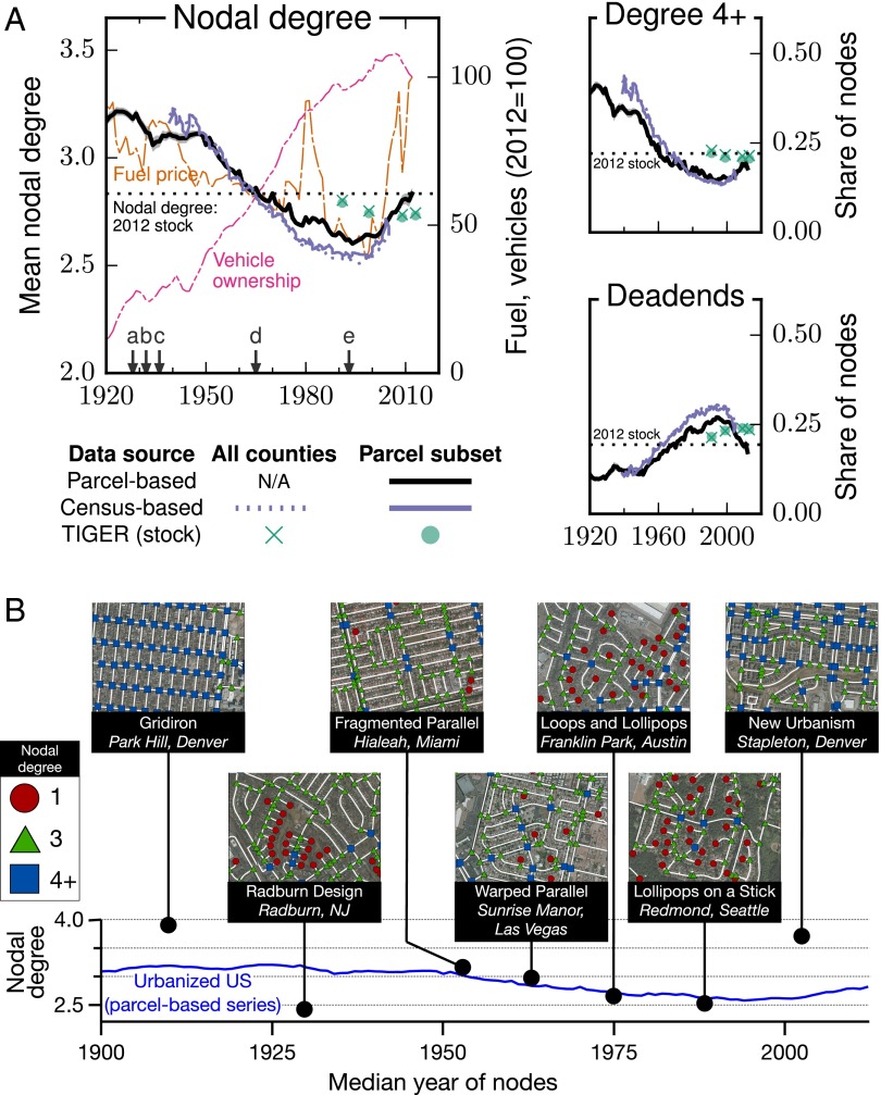
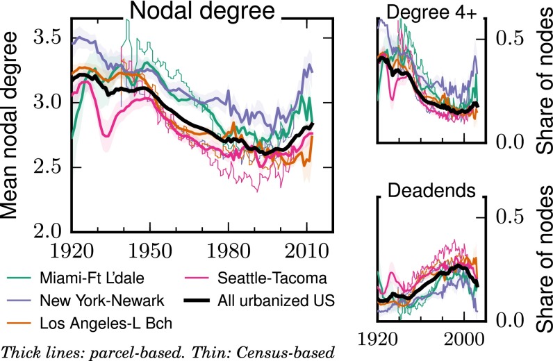
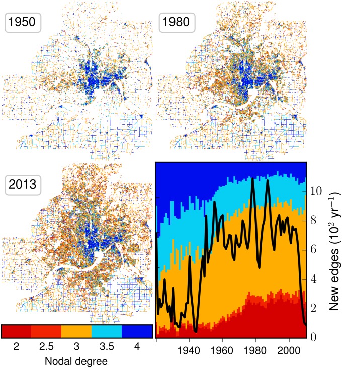
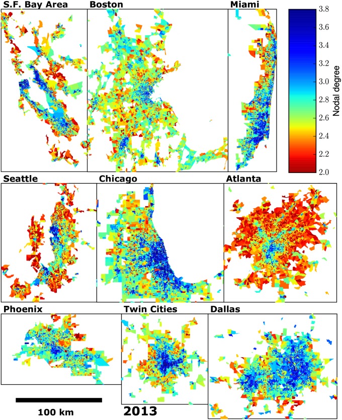
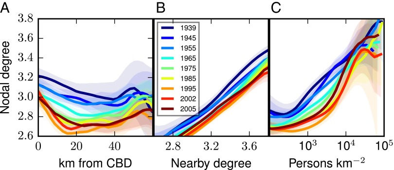
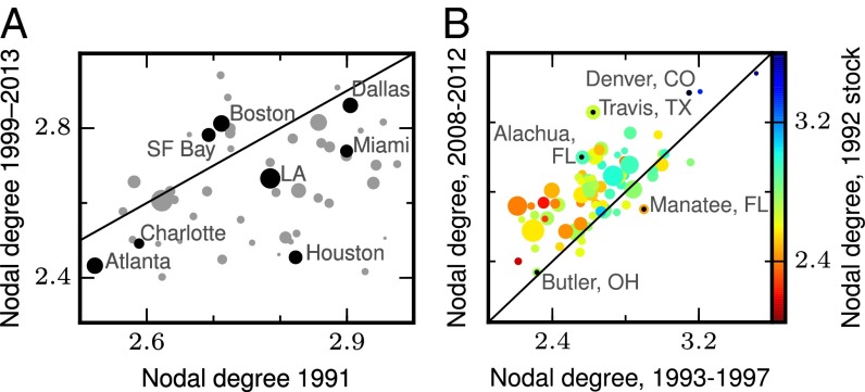
The urban street network is one of the most permanent features of cities. Once laid down, the pattern of streets determines urban form and the level of sprawl for decades to come. We present a high-resolution time series of urban sprawl, as measured through street network connectivity, in the United States from 1920 to 2012. Sprawl started well before private car ownership was dominant and grew steadily until the mid-1990s. Over the last two decades, however, new streets have become significantly more connected and grid-like; the peak in street-network sprawl in the United States occurred in ∼ 1994. By one measure of connectivity, the mean nodal degree of intersections, sprawl fell by ∼ 9% between 1994 and 2012. We analyze spatial variation in these changes and demonstrate the persistence of sprawl. Places that were built with a low-connectivity street network tend to stay that way, even as the network expands. We also find suggestive evidence that local government policies impact sprawl, as the largest increases in connectivity have occurred in places with policies to promote gridded streets and similar New Urbanist design principles. We provide for public use a county-level version of our street-network sprawl dataset comprising a time series of nearly 100 y.

Keywords: climate; policy; road network; transportation; urban sprawl.

Fig. 1.

Trends over time, US urbanized areas 1920–2012. Clearly evident are the rise in sprawl through most of the 20th century, the correlation with archetypal street designs, and the decline in sprawl since the mid-1990s. (A) The three measures of sprawl exhibit similar trends, with street networks becoming increasingly sprawl-like from 1950 through sprawl’s peak in 1994. The 95% confidence intervals are shaded or too narrow to be discernible. Our preferred time series is parcel-based, represented by the solid black lines. As described in Materials and Methods, we validate our findings using two alternative time series, which show broad agreement. A 5-y rolling mean is used before 1950. Also indicated in the Upper panel are key policy events noted in ref. : (a) the Radburn design, (b) report by the Committee on Subdivision Layout, (c) report by the Federal Housing Administration, (d) report by the Institute for Transportation Engineers, and (e) founding of the Congress for the New Urbanism. (B) We identify empirical examples of the five archetypal street design patterns described in ref. and show that the nodal degree of these examples generally matches the overall trends. Location names refer to the approximate neighborhood or city (e.g., Park Hill) and the metropolitan area (e.g., Denver). We also illustrate the 1928 Radburn design and the recent New Urbanist development of Stapleton, which represent opposite extremes in terms of street connectivity. A widespread move toward New Urbanism would eventually restore levels of sprawl to early 20th century levels. Underlying images courtesy of ESRI/Digital Globe.

Fig. 2.

Trends over time, selected metropolitan areas. Trends at the metropolitan area level largely mirror those for the United States as a whole. Data are for CSAs designated by the US Census Bureau. We focus on results from our parcel-based dataset (thicker lines, with 95% confidence intervals shaded), which only provides partial coverage of each CSA. However, similar results are obtained using our Census-based dataset (thinner lines), which is shown for comparison and covers all counties in a given CSA. Note: Before 1980, a 5-y rolling mean is used.

Fig. 3.

Spatial and temporal patterns of sprawl in the Minneapolis–St. Paul region. Individual edges—that is, road segments bounded by two intersections—are shown at three time points. Edges are colored in five categories according to their connectivity, ranging from highly connected (gridded) in blue to cul-de-sacs in red. Connectivity is measured by the mean degree of an edge’s two terminal intersections, explained in the text. Because nodes can be cul-de-sacs, degree three, or degree four-plus, there are five possible values of edge degree, ranging from 2.0 to 4.0. In 1950, the developed area is largely gridded, but growth by 1980 and by 2013 is largely of the low-connectivity kind. Rural roads also tend to be gridded. The Lower Right panel shows the fraction, indicated by the vertical extent of a color, of each edge type built each year. The black line shows the pace of construction, defined as the number of edges dated to each year. Dramatic drops are evident during the Depression, World War II, oil shocks, a recession in the 1970s and 1980s, and the recent Global Financial Crisis. We focus on Minneapolis–St. Paul because all seven central counties are included in our parcel-based data and because the region closely tracks national trends (SI Appendix, Fig. S6).

Fig. 4.

Mean nodal degree in selected metropolitan areas. We find stark variation across metropolitan areas both in the stock and (shown in SI Appendix) in recent construction. Mean nodal degree of street networks is shown for census block groups of selected metropolitan areas in 2013.

Fig. 5.

Uniformity of shifts in sprawl. Nonparametric estimates of the connectivity of roads (mean degree of intersections) as a function of their distance from city center (A), of the mean nodal degree within 1 km in 2013 (B), and of the local population density (C). Over time the relationships fall roughly uniformly and then rise again. Shaded bands show 95% confidence intervals. Values are national averages from our parcel dataset.

Fig. 6.

Persistence of sprawl. (A) Nodal degree of new development, 1999–2013, against nodal degree of the stock (1991), by CSA. Labeled points are highlighted in a darker shade. Most metropolitan regions lie below the 45° line, indicating that the sprawl of the stock increased between 1999 and 2013, but as discussed in Sprawl’s Rise and Decline, this is consistent with a turnaround in the connectivity of new construction given that the stock includes many gridded neighborhoods built before the era of mass car ownership. Data (TIGER-based series) are the same as SI Appendix, Table S1. (B) Nodal degree of new development, 2008–12 versus 1993–97. These time periods represent, respectively, the most recent years in our parcel-based dataset and the time when sprawl was at its peak in ∼1993–97. Colors denote the stock of sprawl in 1992 and demonstrate the persistence of sprawl; counties that had high nodal degree in 1992, and also in the 1993–97 period, were more likely to continue to build connected streets in 2008–12. Also, almost all counties lie above the 45° line, indicating a turnaround in the connectivity of new development. Data (parcel-based series for a subset of counties) are the same as SI Appendix, Table S2.

References

1. Siedentop S, Fina S. Who sprawls most? Exploring the patterns of urban growth across 26 European countries. Environment and Planning – Part A. 2012;44(11):2765–2784.
1. Seto KC, Sánchez-Rodríguez R, Fragkias M. The new geography of contemporary urbanization and the environment. Annu Rev Environ Resour. 2010;35(1):167–194.
1. Ewing R, Cervero R. Travel and the built environment. J Am Plann Assoc. 2010;76(3):265–294.
1. Seto K, et al. Climate Change 2014: Mitigation of Climate Change. Contribution of Working Group III to the Fifth Assessment Report of the Intergovernmental Panel on Climate Change. Cambridge Univ Press; Cambridge, UK: 2014. Human settlements, infrastructure and spatial planning.
1. Glaeser E. Triumph of the City: How Our Greatest Invention Makes Us Richer, Smarter, Greener, Healthier and Happier. Macmillan; Basingstoke, UK: 2011.
Publication types
MeSH terms
LinkOut - more resources