Neuronal variability in orbitofrontal cortex during economic decisions

Abstract

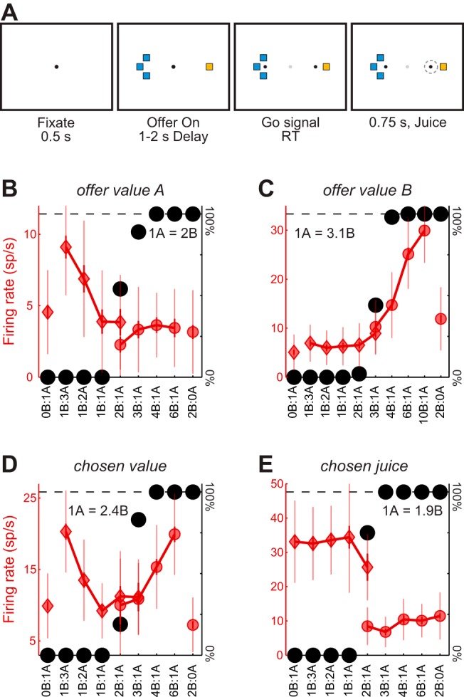
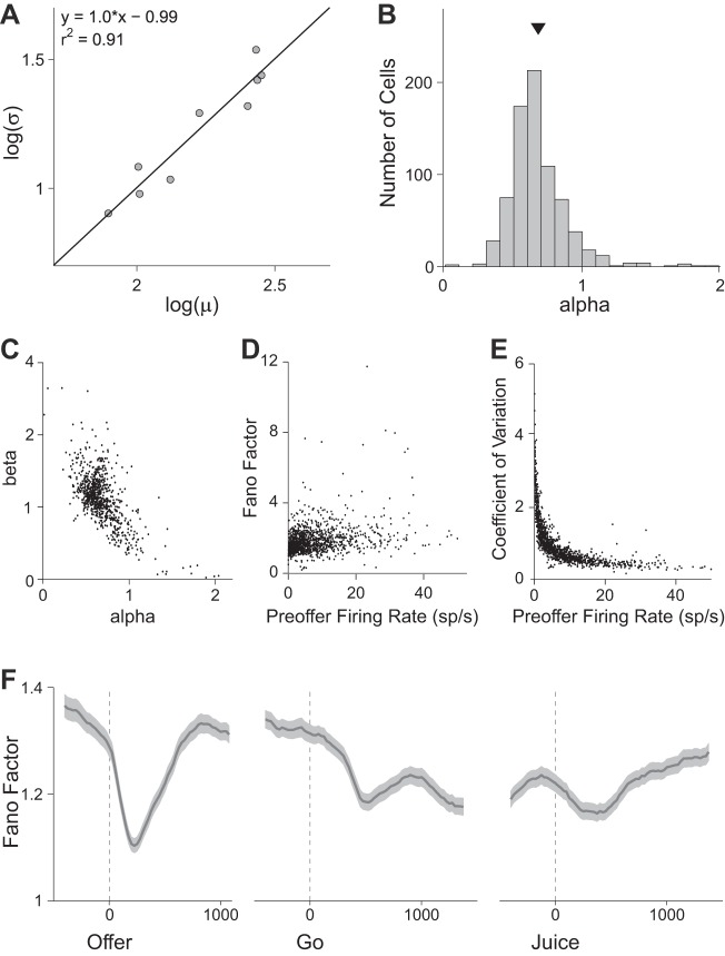
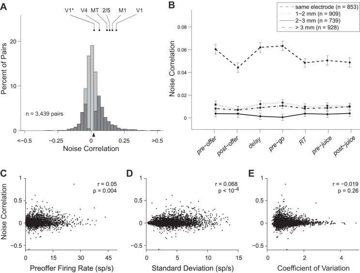
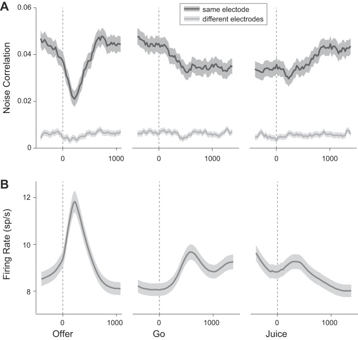
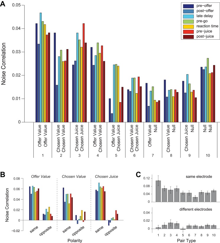
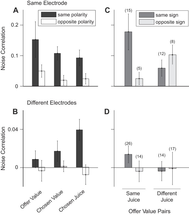
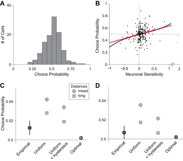
Neuroeconomic models assume that economic decisions are based on the activity of offer value cells in the orbitofrontal cortex (OFC), but testing this assertion has proven difficult. In principle, the decision made on a given trial should correlate with the stochastic fluctuations of these cells. However, this correlation, measured as a choice probability (CP), is small. Importantly, a neuron's CP reflects not only its individual contribution to the decision (termed readout weight), but also the intensity and the structure of correlated variability across the neuronal population (termed noise correlation). A precise mathematical relation between CPs, noise correlations, and readout weights was recently derived by Haefner and colleagues (Haefner RM, Gerwinn S, Macke JH, Bethge M. Nat Neurosci 16: 235-242, 2013) for a linear decision model. In this framework, concurrent measurements of noise correlations and CPs can provide quantitative information on how a population of cells contributes to a decision. Here we examined neuronal variability in the OFC of rhesus monkeys during economic decisions. Noise correlations had similar structure but considerably lower strength compared with those typically measured in sensory areas during perceptual decisions. In contrast, variability in the activity of individual cells was high and comparable to that recorded in other cortical regions. Simulation analyses based on Haefner's equation showed that noise correlations measured in the OFC combined with a plausible readout of offer value cells reproduced the experimental measures of CPs. In other words, the results obtained for noise correlations and those obtained for CPs taken together support the hypothesis that economic decisions are primarily based on the activity of offer value cells.

Keywords: neoroeconomics; subjective value; value-based decision.

Fig. 1.

Behavioral task and cell groups. A: juice choice task. At the beginning of each trial, the animal fixated on the center of a screen. Two sets of colored squares, representing the two offers, appeared after 0.5 s. For each offer, the color indicated the juice identity, and the no. of squares indicated the juice quantity. The animal maintained center fixation for a randomly variable delay (1–2 s), after which the fixation point disappeared, and two saccade targets appeared by the offers (go cue). The animal indicated its choice with a saccade and maintained peripheral fixation for 0.75 s before juice delivery. B: neuron encoding the offer value A. The x-axis represents different offer types ranked by the ratio #B:#A. Black symbols represent the percent of “B” choices. Red symbols represent the neuronal firing rate (diamonds and circles indicate, respectively, choices of juice A and juice B). To highlight the variability in firing rates, thinner error bars here indicate the SD, and thicker error bars indicate the SE. C: neuron encoding the offer value B. D: neuron encoding the chosen value. E: neuron encoding the chosen juice. All conventions C–E are as in B.

Fig. 2.

Neuronal variability in the orbitofrontal cortex (OFC). A: relation between mean firing rate (μ) and variance (σ) for one representative offer value cell (postoffer time window). Data are plotted in log scale, and each data point represents one trial type. The line is obtained from Deming's regression. For this response, α_w = 1.0 and β_w = −0.99. For each tuned cell (763 cells total), α and β were obtained averaging α_w and β_w across time windows. B: distribution of α. Across the population, mean(α) = 0.679 ± 0.008 (SE). C: relation between α and β. Each data point represents one neuron, and the two quantities are strongly anticorrelated. One outlier fell outside the range shown. D: relation between the Fano factor and the baseline activity. Baseline activity was defined as the firing rate in the preoffer time window. Each data point represents one neuron. Across the population, mean(Fano factor) = 1.8. E: relation between coefficient of variation (c_v) and baseline activity. The two quantities are strongly anticorrelated. Across the population, mean(c_v) = 1.0. F: time course of neuronal variability. Dark lines and shaded regions represent, respectively, the mean Fano factor and the corresponding SE (in sp/s). The Fano factor was calculated in 200-ms sliding windows. Neuronal variability dropped sharply shortly after the offer onset; it returned to the initial levels 500–700 ms after the offer; it decreased again and more mildly following the go signal and remained depressed until the trial end. The coefficient of variation presented a similar time course (data not shown).

Fig. 3.

Noise correlation (r_noise) between pairs of neurons in OFC. A: overall distribution of r_noise. In this plot, we pooled all cell pairs and all time windows. Cell pairs with significant r_noise are indicated in dark. The r_noise differed significantly from zero for 1,592/3,439 (46%) cell pairs (P < 0.05; bootstrap analysis; see materials and methods). The black triangle below the x-axis marks the population average. For comparison, we indicate measures of noise correlation previously reported for middle temporal (MT) (Zohary et al. 1994), parietal areas 2/5 (Lee et al. 1998), M1 (Lee et al. 1998), V4 (Mitchell et al. 2009), and V1. For V1, the higher data point shown here is from Poort and Roelfsema (2009), and comparable measures were reported (Gutnisky and Dragoi 2008; Kohn and Smith 2005; Nienborg and Cumming 2006; Smith and Kohn 2008); the lower data point is from Ecker et al. (2010), and a comparable measure was reported (Ecker et al. 2014). B: values of r_noise grouped by interelectrode distance. The x-axis represents different time windows (see materials and methods). For all time windows, r_noise was significantly higher when the two cells were recorded from the same electrode. Notably, r_noise did not decrease beyond values measured at 1-mm distance. Error bars indicate SE. C: noise correlation as a function of the geometric mean of baseline firing rates. The geometric mean averaged across the population was 5.85 ± 0.09 sp/s (mean ± SE). Across the population, noise correlations were weakly but significantly correlated with the geometric mean of baseline firing rates (r = 0.05, P < 0.005; Spearman rank correlation). D: noise correlation as a function of the geometric mean of SDs. Population mean ± SE = 4.20 ± 0.04 sp/s. E: noise correlation as a function of the geometric mean of the coefficients of variation. Population mean ± SE = 1.048 ± 0.009. Data for C–E were taken from the preoffer time window. Note that values of r_noise for individual cell pairs fluctuate throughout the course of the trial and are negatively correlated with firing rate across time windows (see Fig. 4).

Fig. 4.

Time course of noise correlation and firing rate. A: noise correlation. Values of r_noise were computed in 200-ms time windows slid by 25-ms intervals around offer presentation (left), go signal (middle), and juice delivery (right). Each data point is placed on the x-axis in the center of the corresponding time window. Dark lines and shaded regions indicate mean(r_noise) and SE, respectively. Noise correlations dropped sharply and transiently after the offer. This effect, most evident when neurons were recorded from the same electrode, was also observed when neurons were recorded from different electrodes. A second and more modest decrease in r_noise occurred after the go signal. This second drop was pronounced only in same-electrode pairs. Noise correlations gradually returned to baseline levels after juice delivery. All cell pairs in the dataset are included (863 same-electrode pairs, dark gray; 2,576 different-electrode pairs, light gray). B: firing rate. Shown is the firing rate averaged across all tuned cells (763 cells). All conventions as in A.

Fig. 5.

Noise correlations for different pair types. A: mean r_noise recorded for 10 pair types and 7 time windows. The no. of pairs for each pair type is indicated in Table 1, and colors indicate different time windows. Pooling time windows, r_noise varied significantly across pair type (P < 10⁻³, 1-way ANOVA). Post hoc tests found several significant differences in r_noise: type 1 > types 6–10, type 2 > types 7–9, type 3 > types 6–8, type 4 > types 7–9, and type 10 > types 7–8 (all P < 0.05, Tukey's least-significant difference). We also observed consistent trends across time windows. Starting from the preoffer time window (baseline), r_noise decreased in the postoffer time window. It then increased in the delay and pre-go time windows compared with the postoffer. It decreased again in the reaction time time window and remained roughly stable for the rest of the trial. These trends were observed for all pair types (with the exception of pair type 3 in the preoffer time window; see main text). B: mean r_noise for pair types 1-3, divided by juice polarity (see materials and methods). Pairs of neurons with the same polarity are on the left of each panel, while those with opposite polarities are on the right. For chosen juice pairs with opposite polarity, residual activity from the previous trial leads to negative noise correlations in the preoffer time window. C: mean r_noise by pair type. Data from different time windows are averaged separately for cell pairs recorded from the same electrode (top) and from different electrodes (bottom). All error bars indicate SE.

Fig. 6.

Noise correlations depend on the polarity of the two cells. A and C: cell pairs from the same electrode. B and D: cell pairs from different electrodes. A and B: noise correlations between cells in the same group (offer value, chosen value, and chosen juice). Black (white) bars refer to pairs of cells with the same (opposite) polarity. For each cell group, r_noise was higher when the two neurons had the same polarity. This observation was true both at short and long distance. C and D: noise correlations between pairs of offer value cells. Pairs were divided in 8 pools depending on whether the two cells were recorded from the same or different electrode (top, bottom), on whether the two neurons encoded the same juice or different juices (left, right), and on whether the sign of the encoding for the two cells was the same or different (dark gray, light gray). In general, r_noise was highest when two cells encoded the same juice with the same sign. Values of r_noise show the average across all time windows. Nos. in parentheses indicate the no. of neurons in each pool. All error bars indicate SE.

Fig. 7.

Choice probabilities and noise correlations. A: empirical distribution of CPs measured in the 500 ms after offer onset (N = 229 cells). Cells with positive and negative encoding were pooled (see materials and methods). Across the population, mean(CP) = 0.513 ± 0.007 (SE). B: relation between CP and neuronal sensitivity. Each data point represents one offer value cell. For each neuron, the neuronal sensitivity was calculated dividing the tuning slope by the average SD. Cells encoding the two juices (A and B) were pooled, but cells with negative encoding were not rectified here (sensitivity < 0). Color lines indicate the result of a linear fit (a₀ + a₁x; red line) and the result of a fit based on a third-order polynomial (a₀ + a₁x + a₂x² + a₃x³; blue line). In the latter, terms a₀ and a₁ were significantly >0, while terms a₂ and a₃ were indistinguishable from 0, indicating that the readout of offer value cells was close to optimal (Haefner et al. 2013). Two outliers (gray dots) were not included in the regressions, but adding them to the dataset did not alter any of the significance results. C and D: reconstructing choice probabilities from noise correlations. Each data point represents the mean(CP) obtained empirically or from a simulation (see results). The error bars shown for the empirical measure indicate SE. For each readout scheme, long-distance and mixed-distance simulations provided, respectively, a lower bound and an upper bound for mean(CP) (see materials and methods). Empirical and simulated CP were calculated during the postoffer time window (C) and the window 150–400 ms following offer onset (D).

References

1. Abbott LF, Dayan P. The effect of correlated variability on the accuracy of a population code. Neural Comput 11: 91–101, 1999. - PubMed
1. Ahn S, Fessler JA. Globally convergent image reconstruction for emission tomography using relaxed ordered subsets algorithms. IEEE Trans Med Imaging 22: 613–626, 2003. - PubMed
1. Averbeck BB, Lee D. Neural noise and movement-related codes in the macaque supplementary motor area. J Neurosci 23: 7630–7641, 2003. - PMC - PubMed
1. Bair W, Koch C. Temporal precision of spike trains in extrastriate cortex of the behaving macaque monkey. Neural Comput 8: 1185–1202, 1996. - PubMed
1. Britten KH, Newsome WT, Saunders RC. Effects of inferotemporal cortex lesions on form-from-motion discrimination in monkeys. Exp Brain Res 88: 292–302, 1992. - PubMed
Publication types
LinkOut - more resources