Choosing the Most Effective Pattern Classification Model under Learning-Time Constraint

Abstract

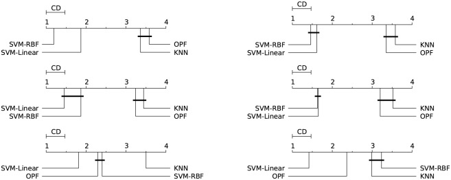
Nowadays, large datasets are common and demand faster and more effective pattern analysis techniques. However, methodologies to compare classifiers usually do not take into account the learning-time constraints required by applications. This work presents a methodology to compare classifiers with respect to their ability to learn from classification errors on a large learning set, within a given time limit. Faster techniques may acquire more training samples, but only when they are more effective will they achieve higher performance on unseen testing sets. We demonstrate this result using several techniques, multiple datasets, and typical learning-time limits required by applications.

Fig 1. Example of interactive graph-based image segmentation.

(a) The user draws labeled markers (a training set) inside and outside the object, and segmentation is based on optimum path competition from the markers in an image graph. (b) Image segmentation first relies on a pixel classifier, which is trained from the markers to create a fuzzy object map (the object should appear brighter than the background). (c) Second, the image is interpreted as a graph, whose arc weights should be lower on the border of the object than elsewhere. (d)-(f) The visual feedback from these results guides the user to the image location where more markers must be selected, improving fuzzy object map, arc weights, and so segmentation along a few interventions.

Fig 2. Correlation table between each pair of training sets, 𝓩₁, after the learning process with learning constraint of 300 seconds.

Cod-RNA (a—d). Connect (e—h). Covertype (i—l). IJCNN (m—p). SensIT (q—t).

Fig 3. Cod-RNA.

Comparison of all classifiers against each other with the Nemenyi test and learning time constraint equals to 1, 5, 20, 60, 300, and 1200 seconds. Groups of classifiers that are not significantly different (at p = 0.05) are connected.

Fig 4. Connect-4.

Comparison of all classifiers against each other with the Nemenyi test and learning time constraint equals to 1, 5, 20, 60, 300, and 1200 seconds. Groups of classifiers that are not significantly different (at p = 0.05) are connected.

Fig 5. Covertype.

Comparison of all classifiers against each other with the Nemenyi test and learning time constraint equals to 1, 5, 20, 60, 300, and 1200 seconds. Groups of classifiers that are not significantly different (at p = 0.05) are connected.

Fig 6. IJCNN 2001.

Comparison of all classifiers against each other with the Nemenyi test and learning time constraint equals to 1, 5, 20, 60, 300, and 1200 seconds. Groups of classifiers that are not significantly different (at p = 0.05) are connected.

Fig 7. SensIT Vehicle (combined).

Comparison of all classifiers against each other with the Nemenyi test and learning time constraint equals to 1, 5, 20, 60, 300, and 1200 seconds. Groups of classifiers that are not significantly different (at p = 0.05) are connected.

Fig 8. Randomly selected samples in the final training set when using the Cone-Torus dataset.

(a) k-NN and 1 sec. (b) OPF and 1 sec. (c) LSVM and 1 sec. (d) KSVM and 1 sec. (e) k-NN and 1.5 sec. (f) OPF and 1.5 sec. (g) LSVM and 1.5 sec. (h) KSVM and 1.5 sec.

Fig 9. Selected samples by each classification model in the final training set, when using the Cone-Torus dataset and time limit of 1s.

(a) k-NN. (b) OPF. (c) LSVM. (d) KSVM.

References

-
- Suzuki CTN, Gomes JF, Falcão AX, Shimizu SH, Papa JP. Automated Diagnosis of Human Intestinal Parasites using Optical Microscopy Images. In: Proceedings of the International Symposium on Biomedical Imaging: From Nano to Macro (ISBI). IEEE; 2013. p. 460–463.
- Souza A, Falcão AX, Ray L. 3-D Examination of Dental Fractures From Minimum User Intervention. In: Proceedings of SPIE on Medical Imaging: Image-Guided Procedures, Robotic Interventions, and Modeling. vol. 8671; 2013. p. 86712K–86712K–8.
- Spina TV, Falcão AX, de Miranda PAV. Intelligent Understanding of User Interaction in Image Segmentation. International Journal of Pattern Recognition and Artificial Intelligence (IJPRAI). 2012;26(2):1265001–1–1265001–26. 10.1142/S0218001412650016 - DOI
- Jain AK, Duin RPW, Mao J. Statistical Pattern Recognition: A Review. IEEE Transactions on Pattern Analysis and Machine Intelligence (TPAMI). 2000;22(1):4–37. 10.1109/34.824819 - DOI
Publication types
MeSH terms
LinkOut - more resources
Full Text Sources
Other Literature Sources