fMRI Analysis-by-Synthesis Reveals a Dorsal Hierarchy That Extracts Surface Slant

Abstract

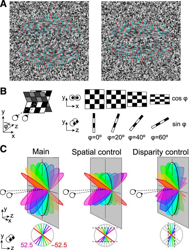
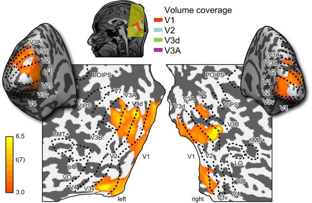
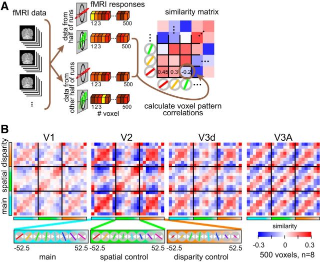
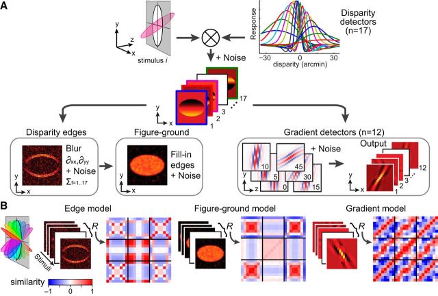
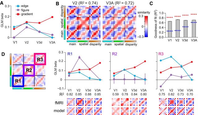
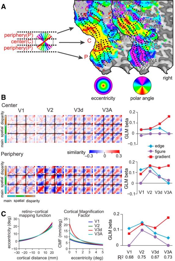
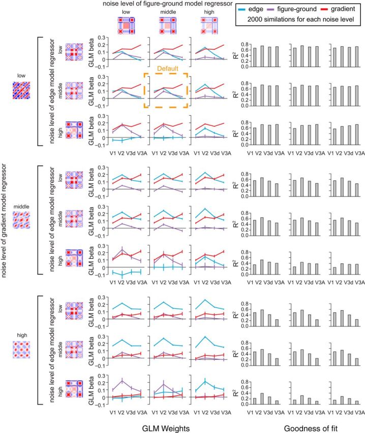
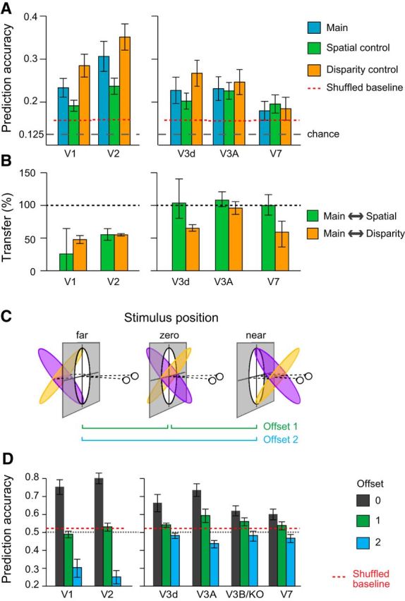
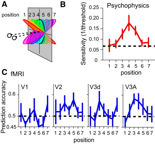
The brain's skill in estimating the 3-D orientation of viewed surfaces supports a range of behaviors, from placing an object on a nearby table, to planning the best route when hill walking. This ability relies on integrating depth signals across extensive regions of space that exceed the receptive fields of early sensory neurons. Although hierarchical selection and pooling is central to understanding of the ventral visual pathway, the successive operations in the dorsal stream are poorly understood. Here we use computational modeling of human fMRI signals to probe the computations that extract 3-D surface orientation from binocular disparity. To understand how representations evolve across the hierarchy, we developed an inference approach using a series of generative models to explain the empirical fMRI data in different cortical areas. Specifically, we simulated the responses of candidate visual processing algorithms and tested how well they explained fMRI responses. Thereby we demonstrate a hierarchical refinement of visual representations moving from the representation of edges and figure-ground segmentation (V1, V2) to spatially extensive disparity gradients in V3A. We show that responses in V3A are little affected by low-level image covariates, and have a partial tolerance to the overall depth position. Finally, we show that responses in V3A parallel perceptual judgments of slant. This reveals a relatively short computational hierarchy that captures key information about the 3-D structure of nearby surfaces, and more generally demonstrates an analysis approach that may be of merit in a diverse range of brain imaging domains.

Keywords: 3-D vision; binocular disparity; fMRI; slant.

Figure 1.

Stimulus illustrations. A, Example random dot stereograms of the slanted discs used in the study rendered as red-cyan anaglyphs. The stimuli depict slants of −37.5° (left) and −52.5° (right) for a participant with an interpupilary spacing of 6.4 cm viewing from a distance of 65 cm. (Note, if viewing without glasses, there might be an apparent blurring of the slanted stimuli that varies with slant angle; this cue was not available when our participants viewed the stimuli in the scanner through spectral comb filters). B, Schematic of the changes that accompany a physical change of slant. C, Diagrams of the parametric slant variations in the three experimental conditions: Main: simulated rotation of a physical disc; Spatial control: projection height in the image plane was constant as slant was manipulated; Disparity control: the mean (unsigned) disparity was constant as slant was varied.

Figure 2.

Illustrations of the cortical surface with superimposed locations of the ROIs. Sulci are depicted in darker gray than the gyri. Shown on the maps are retinotopic areas, V3B/KO, the human motion complex (hMT+/ V5), and LO area. The activation map shows the results of a random-effects analysis of a searchlight classifier that discriminated between different slanted stimuli. The color code represents the t value of the classification accuracies obtained by moving a spherical aperture throughout the measured volume. This confirmed that our ROIs covered the likely loci of areas encoding stimulus information.

Figure 3.

Illustration of the cross-correlation approach and empirical data. A, A schematic of the data treatment. The fMRI data were split in halves and the vector of voxel responses was then correlated across stimulus conditions. We used a cross-validation procedure, averaging together the results of different splits of the empirical data. The resulting cross-correlation matrix (averaged over cross-validations) is represented using a blue-to-red color code. B, Empirical cross-correlation matrices from areas V1, V2, V3d, and V3A. Slant angle varies in an ordered fashion for the three experimental conditions (main, spatial control, disparity control). The mean regression coefficient across split-halves is represented by the color saturation of each cell in the matrix.

Figure 4.

Illustration of the modeling approach. A, The disparity stimulus is fed through a bank of disparity filters with noise. The outputs of these filters are then fed to a disparity edge detection algorithm and a set of disparity gradient filters. The results of the disparity edge detection process are used to generate a figure–ground segmentation map. B, The outputs for the three different models are calculated for all of the stimuli presented to the observers. These model outputs are used to create cross-correlation matrices in the same manner as the empirical data.

Figure 5.

Regression analysis of the empirical cross-correlation matrices. A, The weights of each model are plotted for areas V1, V2, V3d, and V3A. B, Model reconstructions based on the GLM β weights calculated in A with 2000 simulations. This result is confirmatory in allowing visualization of the features captured by the modeling approach. C, Goodness of fit of the GLM model in each region of interest with the associated noise ceiling bounds that estimate the minimum and maximum GLM performance that could be achieved given the noise in the data (Nili et al., 2014). The upper bound (red) is calculated by using the between-subjects mean matrix as a regressor for bootstrapped (10,000 samples) resampled averages of the subjects' data. The lower bound (blue) was calculated using single subjects' matrices as regressors for the bootstrapped resampled averages of the subjects' data. In both cases, the bounds were defined as the median value of the boostrapped R² samples. D, GLM analyses conducted within subregions of the cross-correlation matrices. Error bars indicate ±SEM.

Figure 6.

Cross-correlation matrices calculated using fMRI data partitioned into central- and peripheral-regions and taking account of cortical magnification. A, Example flat maps of a hemisphere from one participant showing phase-encoded polar- and eccentricity-based retinotopic maps. We used these maps to partition the cortical regions of interest to localize regions that respond to the central portion of the stimulus and edge locations (shown by the diagram of the partitioned stimulus locations). We then recomputed cross-correlation matrices based on the subdivided regions of interest. B, Model-based GLM analysis of the empirical cross-correlation matrices showing the weights attached to each model in areas V1 to V3A. Error bars (±SEM) lie within plotting symbols. C, Cortical magnification factors (CMFs) were defined separately for each of V1, V2, V3, and V3A using the formulas (Eqs. 4, 5; see Methods and Materials) and parameters estimated from retinotopic mapping data. Visual eccentricity as a function of cortical distance can be approximated by an exponential (left), where we use the 8° eccentricity location as a reference point. CMFs are obtained by computing the derivatives of inverses of these eccentricity representations (middle). The plots were regenerated from Yamamoto et al., (2008). We computed model cross-correlation matrices where the input representations were distorted using cortical magnification factors for each area. We then used these as regressors for the empirical fMRI data, producing the plot of GLM weights (right). Error bars (±SEM) lie within plotting symbols.

Figure 7.

Simulations of the models with different noise parameters. Model-based GLM analysis of the empirical cross-correlation matrices where the three component models (edge, figure-ground and gradient) have their noise levels varied systematically. The default noise parameters used in the main paper are highlighted by the dashed orange box. For the edge and figure-ground models, we ran the simulations by adding normally distributed noise whose SDs were ×0.5 (low noise level), ×1.0 (middle), or ×2.0 (high) of the default level. For the gradient model, noise was ×1.0 (low), ×2.0 (middle), or ×3.0 (high) the default. Bar graphs to the right of the figure plot the R² value of the model fit; their layout corresponds to the line graphs on the left side of the figure.

Figure 8.

Results of MVPA decoding of surface slant. A, Eight-way classification results across ROIs with above chance prediction accuracy for the three conditions. Error bars show ±SEM. The dotted horizontal line represents the upper 97.5^th centile of randomly permuted data. B, Transfer results expressed as a percentage of the within condition prediction accuracy. One-hundred percent would indicate the same accuracy for testing and training between conditions as for testing on the same condition. Error bars show SEM. C, Manipulating the depth positions of the slanted surfaces. Opposing slants were presented centered on the fixation point (zero), or translated away (far) or toward (near) the observer. D, Prediction accuracies for the binary classification of opposing slants. The dashed red line represents the upper 97.5^th centile based on randomly permuted data. Error bars show ±SEM.

Figure 9.

Testing for similarities between perceptual discriminability and fMRI-decoding. A, An illustration of the stimulus slants used for the psychophysical and fMRI measurements. B, Observers' sensitivity to slight changes in slant at different pedestal slants. Thresholds were measured at each of the eight stimulus slants illustrated in A. To compare with the fMRI results, we averaged neighboring pairs together to yield discrimination thresholds at seven positions. The dashed horizontal line corresponds to a slant discrimination threshold of 15° (i.e., the location at which neighboring pairs of stimuli used in the study would only just be discriminable). Error bar shows ±SEM. C, Two-way prediction accuracies for a classifier trained on fMRI data from neighboring slants. Error bars show ±SEM.

References

1. Backus BT, Fleet DJ, Parker AJ, Heeger DJ. Human cortical activity correlates with stereoscopic depth perception. J Neurophysiol. 2001;86:2054–2068. - PubMed
1. Ban H, Preston TJ, Meeson A, Welchman AE. The integration of motion and disparity cues to depth in dorsal visual cortex. Nat Neurosci. 2012;15:636–643. doi: 10.1038/nn.3046. - DOI - PMC - PubMed
1. Bredfeldt CE, Cumming BG. A simple account of cyclopean edge responses in macaque V2. J Neurosci. 2006;26:7581–7596. doi: 10.1523/JNEUROSCI.5308-05.2006. - DOI - PMC - PubMed
1. Brouwer GJ, Heeger DJ. Decoding and reconstructing color from responses in human visual cortex. J Neurosci. 2009;29:13992–14003. doi: 10.1523/JNEUROSCI.3577-09.2009. - DOI - PMC - PubMed
1. Chandrasekaran C, Canon V, Dahmen JC, Kourtzi Z, Welchman AE. Neural correlates of disparity-defined shape discrimination in the human brain. J Neurophysiol. 2007;97:1553–1565. - PubMed
Publication types