Anatomical guidance for functional near-infrared spectroscopy: AtlasViewer tutorial

Abstract

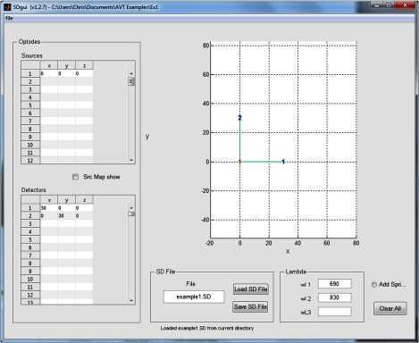
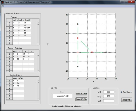
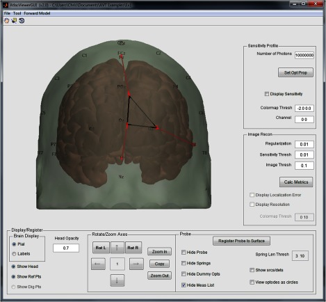
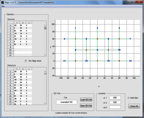
Functional near-infrared spectroscopy (fNIRS) is an optical imaging method that is used to noninvasively measure cerebral hemoglobin concentration changes induced by brain activation. Using structural guidance in fNIRS research enhances interpretation of results and facilitates making comparisons between studies. AtlasViewer is an open-source software package we have developed that incorporates multiple spatial registration tools to enable structural guidance in the interpretation of fNIRS studies. We introduce the reader to the layout of the AtlasViewer graphical user interface, the folder structure, and user files required in the creation of fNIRS probes containing sources and detectors registered to desired locations on the head, evaluating probe fabrication error and intersubject probe placement variability, and different procedures for estimating measurement sensitivity to different brain regions as well as image reconstruction performance. Further, we detail how AtlasViewer provides a generic head atlas for guiding interpretation of fNIRS results, but also permits users to provide subject-specific head anatomies to interpret their results. We anticipate that AtlasViewer will be a valuable tool in improving the anatomical interpretation of fNIRS studies.

Keywords: atlas; image reconstruction; near-infrared spectroscopy; photon migration; probe design; tutorial.

Fig. 1

The AtlasViewer graphical user interface centers around the display of the selected atlas, with the scalp and cortical surfaces visible. By default, the atlas displayed and utilized by AtlasViewer is based on the high-resolution Colin27 atlas. Within the control panels, there are options to adjust the visible atlas components, the viewing angle and zoom, and probe display. The top menu bar items and the use of the sensitivity profile are detailed in the text.

Fig. 2

The initial view of the SDgui, which provides the basic interface to create sources and detectors, set the wavelengths of light being used, and name the “.SD” file. The probe graph in the upper-right portion of the screen provides a visual representation of the probe and provides the interface for creating sensor channels by connecting sources and detectors.

Fig. 3

The SDgui “Add Springs” window allows the user to create spring connections between optodes, create dummy optodes for the sake of positioning or to reinforce the probe geometry, and to anchor optodes to reference points on the head surface.

Fig. 4

The result of registering the example probe to the atlas using the spring relaxation method. The depiction of the probe geometry indicates that the desired spacing was maintained within 3 mm between all source and detector positions (black color coding), while the springs connecting to anchor points are longer than their specified length by more than 10 mm (red color coding). Due to the use of unbalanced anchor points, the probe is positioned slightly to the right of the midline and has rotated slightly clockwise. By choosing different anchor points and/or adding additional anchors and springs, one can make minor adjustments to the probe positioning to get their desired positioning.

Fig. 5

This source–detector (SD) configuration provides a laterally symmetrical geometry with sufficient size to encompass the occipital cortex. The alternating SD-source arrangement provides even coverage over a large area.

Fig. 6

The probe in Fig. 5 is intended for the occipital cortex and will need to curve around the rear of the head. To accomplish this, anchor points 23 and 24 are connected to the probe by weak springs and draw the top corners of the probe along the sides of the head while anchor point 25 explicitly holds the bottom of the probe at a specified distance from the inion reference point “Iz” using a rigid spring.

Fig. 7

(a) The AtlasViewer graphical user interface provides a number of tools for viewing probe geometries: the cortical surface may be colorized using a variety of color maps to depict different anatomical regions, the head surface may have its opacity adjusted or removed entirely, 10-20 reference points may be toggled on/off, the head may be rotated and zoomed, and various elements of the SD file may be hidden or revealed. (b) The popup window that is created when the “Project to cortex” button is pressed contains the list of SD pairs in the measurement list, the channel coordinates in the Monte Carlo space, the channel coordinates in the Montreal Neurological Institute (MNI) space, and a label for the cortical surface that these MNI coordinates correspond to in the segmented atlas volume. Channel coordinates are given at the midpoint between the associated source and detector.

Fig. 8

A sample digpts.txt file is shown. The first five lines are required and define the positions of the five key reference points to determine the affine transformation from the atlas space to the digitized space of the subject. Sources and detectors are defined in the same three-dimensional space as the reference points and are identified as s1, s2, and so on for sources and d1, d2, etc. for detectors. See Ref.  for additional information.

Fig. 9

Running the intersubject variability analysis produces the two figures and table above: (a) shows the various probe optode positions color-coded by subject, (b) represents the standard deviation in millimeters, plotted at the mean of the optode positions, and (c) outputs the data presented in the previous two panels as a table that can be copied to the operating system’s clipboard.

Fig. 10

Running the probe fabrication error analysis also produces two figures and a table. The first figure (not shown) is the same as Fig. 9(a) with the addition of the locations of the original probe design. The second output is shown in (a), which depicts the probe fabrication error. The original optode locations are plotted in black while the digitized optode locations are represented as ellipses plotted at the mean optode location with radii defined by the standard deviation across the subjects along two axes and the color representing the mean-geometric error. (b) Details the AtlasViewer coordinates of the original design and mean locations as well as the mean geometric error.

Fig. 11

(a) The probe in the upper-left panel demonstrates how eight sources and 14 detectors can be arranged to provide moderately even coverage over an $18\times 9{\mathrm{cm}}^2$ rectangle. (b) Using the forward matrix to generate a sensitivity profile, the upper-right panel shows that the resulting probe neatly wraps around the posterior portion of the scalp and provides sufficient coverage of many of the visual cortical regions. (c) The lower-left panel illustrates how 8 sources and 20 detectors can be arranged in a denser geometry, which covers only $10\times 6{\mathrm{cm}}^2$, a reduction in area by a factor of 2.7 compared to the square geometry. (d) The lower-right panel reveals that while the field of view has been significantly decreased, the sensitivity profile within that field is more evenly distributed, which indicates the potential trade-off to be considered in experiment design. The color scale depicts the sensitivity logarithmically from 0.01 to 1.

Fig. 12

(a) The localization error map for the square probe geometry from Sec. 3.1. (b) The resolution map for the same probe. Variation in localization error is highly dependent on the underlying anatomical structure, while probe resolution is predominately a function of source and detector placement. The color scale is linear and spans from 0 to 10 mm as indicated in the “Colormap Thresh” edit box.

References

1. Boas D. A., et al. , “Twenty years of functional near-infrared spectroscopy: introduction for the special issue,” NeuroImage 85(1), 1–5 (2014).NEIMEF10.1016/j.neuroimage.2013.11.033 - DOI - PubMed
1. White B. R., Culver J. P., “Quantitative evaluation of high-density diffuse optical tomography: in vivo resolution and mapping performance,” J. Biomed. Opt. 15(2), 026006 (2010).JBOPFO10.1117/1.3368999 - DOI - PMC - PubMed
1. Zeff B. W., et al. , “Retinotopic mapping of adult human visual cortex with high-density diffuse optical tomography,” Proc. Natl. Acad. Sci. U. S. A. 104(29), 12169–12174 (2007).PNASA610.1073/pnas.0611266104 - DOI - PMC - PubMed
1. Jasper H. H., “The ten-twenty electrode system of the International Federation,” Electroencephalogr. Clin. Neurophysiol. 10, 371–375 (1958). - PubMed
1. Jurcak V., Tsuzuki D., Dan I., “10/20, 10/10, and 10/5 systems revisited: their validity as relative head-surface-based positioning systems,” NeuroImage 34(4), 1600–1611 (2007).NEIMEF10.1016/j.neuroimage.2006.09.024 - DOI - PubMed