

Analytic expressions for ULF wave radiation belt radial diffusion coefficients
- PMID: 26167440
- PMCID: PMC4497482
- DOI: 10.1002/2013JA019204
Analytic expressions for ULF wave radiation belt radial diffusion coefficients
Abstract
We present analytic expressions for ULF wave-derived radiation belt radial diffusion coefficients, as a function of L and Kp, which can easily be incorporated into global radiation belt transport models. The diffusion coefficients are derived from statistical representations of ULF wave power, electric field power mapped from ground magnetometer data, and compressional magnetic field power from in situ measurements. We show that the overall electric and magnetic diffusion coefficients are to a good approximation both independent of energy. We present example 1-D radial diffusion results from simulations driven by CRRES-observed time-dependent energy spectra at the outer boundary, under the action of radial diffusion driven by the new ULF wave radial diffusion coefficients and with empirical chorus wave loss terms (as a function of energy, Kp and L). There is excellent agreement between the differential flux produced by the 1-D, Kp-driven, radial diffusion model and CRRES observations of differential electron flux at 0.976 MeV-even though the model does not include the effects of local internal acceleration sources. Our results highlight not only the importance of correct specification of radial diffusion coefficients for developing accurate models but also show significant promise for belt specification based on relatively simple models driven by solar wind parameters such as solar wind speed or geomagnetic indices such as Kp.
Key points: Analytic expressions for the radial diffusion coefficients are presentedThe coefficients do not dependent on energy or wave m valueThe electric field diffusion coefficient dominates over the magnetic.
Figures
 and
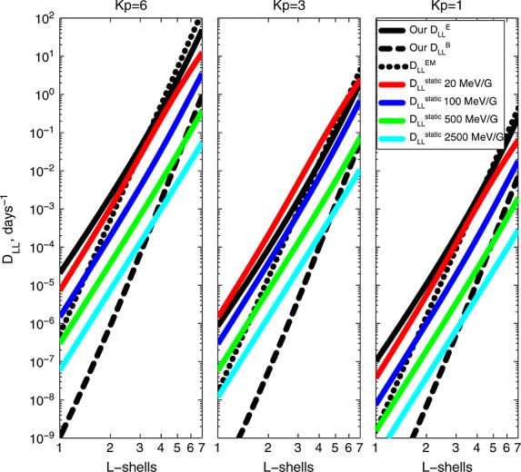
and  , with the electromagnetic
  and electrostatic
  diffusion coefficients presented in Brautigam and Albert [2000]. The black solid, dashed, and dotted lines represent
  ,
,  , and , respectively. The solid red, blue, green, and cyan lines represent the electrostatic diffusion coefficient,
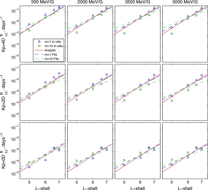
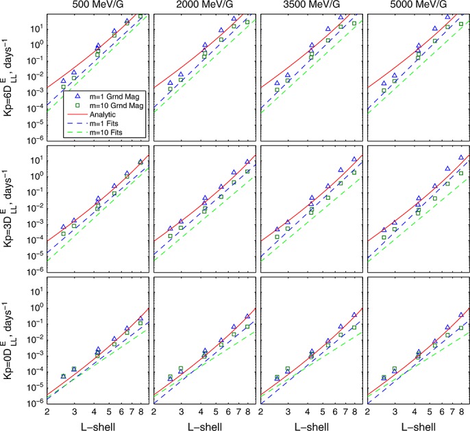
  , for electrons with M values of 20 MeV/G, 100 MeV/G, 500 MeV/G, and 2500 MeV/G, respectively. These M values correspond to a 1 MeV electron in a dipole model of the Earth's magnetic field at L = 1.84, 3.15, 5.38, 6.78, and 9.21, respectively.
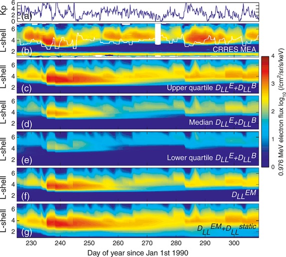
 values from Brautigam and Albert [2000]; and (g) the diffusion model with the and
  values from Brautigam and Albert [2000].
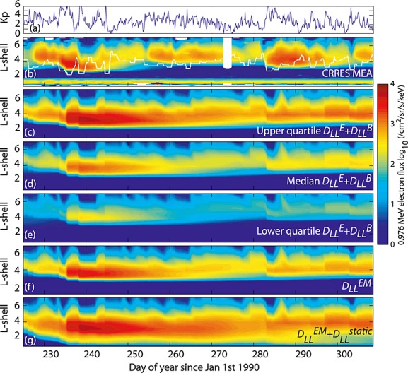
 values from Brautigam and Albert [2000]; and (g) the diffusion model with the
  and
and  values from Brautigam and Albert [2000].
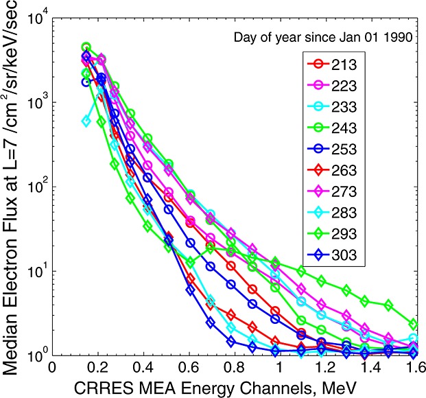
References
-
- Baker DN, Blake JB, Callis LB, Cummings JR, Hovestadt D, Kanekal S, Klecker B, Mewaldt RA. Zwickl RD. Relativistic electron acceleration and decay time scales in the inner and outer radiation belts: Sampex. Geophys. Res. Lett. 1994;21(6):409–412. doi: 10.1029/93GL03532. - DOI
-
- Beutier T. Boscher D. A three-dimensional analysis of the electron-radiation belt by the Salammbo Code. J. Geophys. Res. 1995;100(A8):14,853–14,861. doi: 10.1029/94JA03066. - DOI
-
- Blake JB, Kolasinski WA, Fillius RW. Mullen EG. Injection of electrons and protons with energies of tens of MeV into L < 3 on 24 March 1991. Geophys. Res. Lett. 1992;19(8):821–824. doi: 10.1029/92GL00624. - DOI
-
- Brautigam DH. Albert JM. Radial diffusion analysis of outer radiation belt electrons during the October 9, 1990, magnetic storm. J. Geophys. Res. 2000;105(A1):291–309.
-
- Brautigam DH, Ginet GP, Albert JM, Wygant JR, Rowland DE, Ling A. Bass J. CRRES electric field power spectra and radial diffusion coefficients. J. Geophys. Res. 2005;110:A02214. doi: 10.1029/2004JA010612. - DOI
LinkOut - more resources
Full Text Sources
Other Literature Sources