Quantifying effects of stochasticity in reference frame transformations on posterior distributions

Abstract

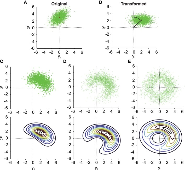
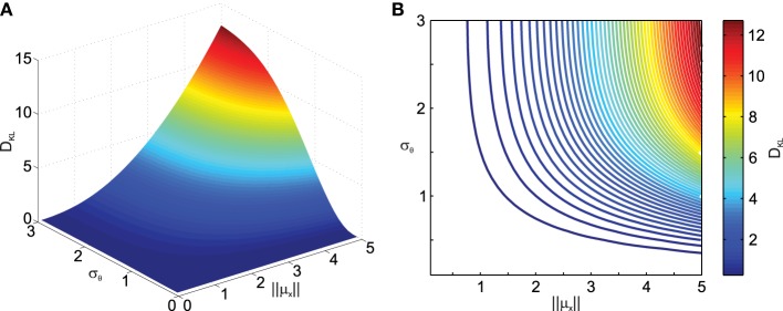
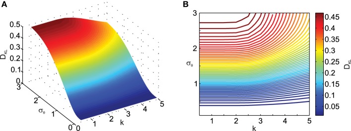
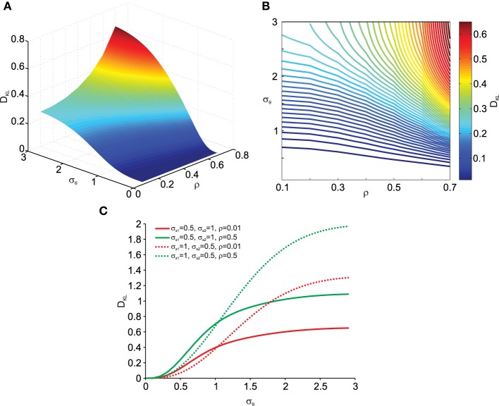
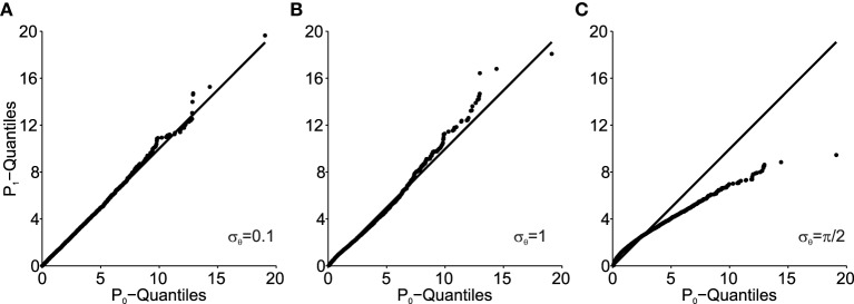
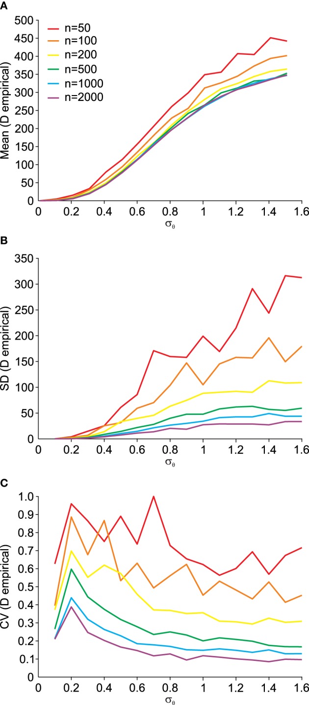
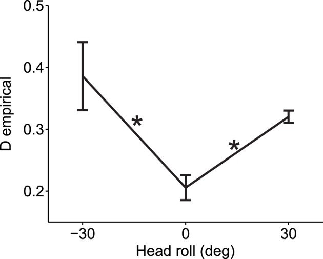
Reference frame transformations are usually considered to be deterministic. However, translations, scaling or rotation angles could be stochastic. Indeed, variability of these entities often originates from noisy estimation processes. The impact of transformation noise on the statistics of the transformed signals is unknown and a quantification of these effects is the goal of this study. We first quantify analytically and numerically how stochastic reference frame transformations (SRFT) alter the posterior distribution of the transformed signals. We then propose an new empirical measure to quantify deviations from a given distribution when only limited data is available. We apply this empirical measure to an example in sensory-motor neuroscience to quantify how different head roll angles change the distribution of reach endpoints away from the normal distribution.

Keywords: Stochastic noise; deviation from normality; reaching; reference frame transformation; sensory-motor transformation.

Figure 1

Noisy rotations. (A) Scatter plot of n = 5000 original normally distributed data points with μ_x1 = 0, μ_x2 = 3, ρ = 0.5 and σ_x1 = σ_x2 = 1. (B) Same data as in (A) rotated by a fixed μ_θ = −π/4. (C–E) (top). Results from noisy rotations of the data in (A) by the same average amount as in (B) (μ_θ = −π/4) but with different rotational standard deviations, i.e., σ_θ = 0.4 (C), σ_θ = 1 (D), σ_θ = π/2 (E). Bottom parts of (C–E) show contour plots of the distribution f_y(y₁, y₂) (Equation 10).

Figure 2

Effect of transformation angle noise σ_θ and data eccentricity from the origin ||μ_x|| on the multi-variate normality of the transformed data, as captured by the Kullback–Leibler distance D_KL (Equation 11). μ_x1 = 0, μ_x2 = 1, ρ = 0.5 and σ_x1 = σ_x2 = 1. (A) Surface plot. (B) Corresponding contour plot.

Figure 3

Effect of transformation angle noise σ_θ and scaling factor k on the multi-variate normality of the transformed data, as captured by the Kullback–Leibler distance D_KL (Equation 11). μ_x1 = 0, μ_x2 = 1, ρ = 0.5 and σ_x1 = σ_x2 = 1. (A) Surface plot. (B) Corresponding contour plot.

Figure 4

Effect of transformation angle noise σ_θ and data correlation ρ on the multi-variate normality of the transformed data, as captured by the Kullback–Leibler distance D_KL (Equation 11). μ_x1 = 0, μ_x2 = 1 and σ_x1 = σ_x2 = 1. (A) Surface plot. (B) Corresponding contour plot. (C) Effect of transformation angle noise σ_θ on D_KL for different combinations of original data variances (σ_x1 and σ_x2) and correlations ρ.

Figure 5

Q–Q plots of the transformed data (P₁) Mahalanobis distance against the original data (P₀) for different values of angular transformation noise σ_θ. (A) σ_θ = 0.1. The Q–Q plot compares an ordered sample distribution with the quantiles of the standard normal distribution. (B) σ_θ = 1. (C) σ_θ = π/2. Deviations from the unity line indicate deviations from normality.

Figure 6

Dependency of the empirical distance D from multi-variate normality (see Equation 14) on the angular transformation noise σ_θ and the number of available data points n. (A) Average (Mean) empirical distance D. (B) Standard deviation (SD) of empirical distance D. (C) Coefficient of variation (CV = SD/Mean) of empirical distance D.

Figure 7

Experimental validation of deviation from normality measure. When the head was rolled and thus a larger reference frame transformation was needed, data deviated more from the normal distribution as compared to when the head was straight (head roll = 0). Average measures across all 7 subjects and across all six reach targets are shown for each head roll angle (means ± s.e.m.). Asterisks indicate significant differences (ANOVA with post-hoc paired t-tests, p < 0.05). Data points at −30 and 30° head roll angle were not significantly different from one another (p > 0.1).

References

1. Blohm G., Crawford J. D. (2007). Computations for geometrically accurate visually guided reaching in 3-d space. J. Vis. 7, 1–22. 10.1167/7.5.4 - DOI - PubMed
1. Buneo C. A., Andersen R. A. (2006). The posterior parietal cortex: sensorimotor interface for the planning and online control of visually guided movements. Neuropsychologia 44, 2594–2606. 10.1016/j.neuropsychologia.2005.10.011 - DOI - PubMed
1. Burdenski T. K. (2000). Evaluating univariate, bivariate, and multivariate normality using graphical procedures. Mult. Lin. Regression Viewpoints 26, 15–28.
1. Burns J. K., Blohm G. (2010). Multi-sensory weights depend on contextual noise in reference frame transformations. Front. Hum. Neurosci. 4:221. 10.3389/fnhum.2010.00221 - DOI - PMC - PubMed
1. Burns J. K., Nashed J. Y., Blohm G. (2011). Head roll influences perceived hand position. J. Vis. 11:3. 10.1167/11.9.3 - DOI - PubMed
LinkOut - more resources