Single-trial dynamics of motor cortex and their applications to brain-machine interfaces

Abstract

Increasing evidence suggests that neural population responses have their own internal drive, or dynamics, that describe how the neural population evolves through time. An important prediction of neural dynamical models is that previously observed neural activity is informative of noisy yet-to-be-observed activity on single-trials, and may thus have a denoising effect. To investigate this prediction, we built and characterized dynamical models of single-trial motor cortical activity. We find these models capture salient dynamical features of the neural population and are informative of future neural activity on single trials. To assess how neural dynamics may beneficially denoise single-trial neural activity, we incorporate neural dynamics into a brain-machine interface (BMI). In online experiments, we find that a neural dynamical BMI achieves substantially higher performance than its non-dynamical counterpart. These results provide evidence that neural dynamics beneficially inform the temporal evolution of neural activity on single trials and may directly impact the performance of BMIs.

Figure 1. Incorporating dynamics into trajectory estimation.

(a) An illustration of a cannonball being fired at dusk, following a parabolic trajectory (orange) according to physical dynamical laws. Photo courtesy Christine Wong. (b,c) The flight of the cannonball is recorded by a low-resolution video camera. However, two factors obscure the true path of the cannonball. First, the camera is low resolution, only being able to capture hundreds of pixels with poor colour resolution. Second, the incoming photons are characterized by Poisson noise, which in part corrupts the image. As a result, the trajectory path recorded in the video might appear very noisy, as illustrated by the dotted-blue trajectory. (d) By incorporating knowledge of Newtonian mechanics, z_k=Fz_k−1, we can arrive at a better estimate of the flight path of the ball. This estimate incorporates knowledge of the laws of motion, the theory of gravity, and air resistance. For example, the ball should not defy gravity by floating up while it is falling. (e) An illustrative analogue of the cannonball in a 2D projection of neural state space. In this toy example, the arrows indicate the dynamics of the neural state, so that for the purposes of this illustration, it rotates counterclockwise. When the dynamics are not taken into account, the neural state trajectory inferred only from noisy single-trial neural observations may be very noisy (blue trace). However, the neural state trajectory noise may be ameliorated by accounting for the neural state dynamics (orange trace). (f) One way in which dynamical information may be included is to linearly weigh the predicted neural state, as a result of a dynamical model and the neural ‘innovations', which is derived from the neural observations. The relative weight given to the dynamical process versus the observation process is influenced by factors such as their noise processes. The relative weight of the contribution from the dynamical process versus the neural innovations is reported in the Results.

Figure 2. Trajectories of the neural state.

(a) Trajectories of the condition-averaged neural data are shown using jPCA, which finds planes that capture rotational structure in the data. The jPCs are rotations of the principal components. (b) Trajectories of a dynamical neural state, inferred by a Kalman filter using cross-validation data, for center-out-and-back reaching. These trajectories are the averages of single trials (s.e.m. shown in shading). Also shown are the dynamics of the learned dynamical system. During the center-out epoch, the trajectories appear to follow the dynamical flow fields. Moreover, during the hold epoch, the strength of the flow field appears weaker. It is worth noting that because the dynamics shown are only 2-dimensional, they are far less rich than the 20-dimensional dynamics and may not adequately capture the dynamics of all portions of the reach (such as during the back-to-center epoch). (c) Behavioural kinematics (hand position) on single trials of Monkey J performing the center-out-and-back task (Methods). (d) The single-trial neural trajectories corresponding to the same single-trial reaches in c.

Figure 3. Neural dynamics accentuate the dynamic range of velocities in hold versus reach.

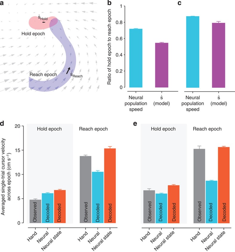
Bar plots in this figure represent the average across seven experimental days in Monkey J and six experimental days in Monkey L, and the error bars denote the s.e.m. (a) A 2D illustration of neural state trajectory regions during the hold and reach epochs, as well as the dynamics they obey. The goal of this analysis is to assess the relationship between . (b) The ratio of the (high-dimensional) neural population speed during the hold epoch to the reach epoch is 0.72 (blue), indicating that the rate of change of the neural population activity is less in the hold epoch than in the reach epoch. The dynamical model captures this feature, with the ratio of the neural state speed predicted by the model in the hold epoch to those in the reach epoch being 0.55 (purple). (c) Same as (b), but for Monkey L. The ratio of the high-dimensional neural velocities is 0.88; the ratio of the model-predicted neural state velocities is 0.79. (d) The averaged single-trial hand velocities during the hold and reach epochs are shown in grey. The average of the decoded single-trial velocities during the hold epoch are comparably low for both the high-dimensional neural data (y_k, blue bar) and the dynamical neural state (s_k, orange bar). However, during the reach epoch, the dynamical neural state is able to decode significantly higher velocities. (e) Same as (d) but for Monkey L.

Figure 4. Decoding with a dynamical neural state as opposed to noisy neural observations.

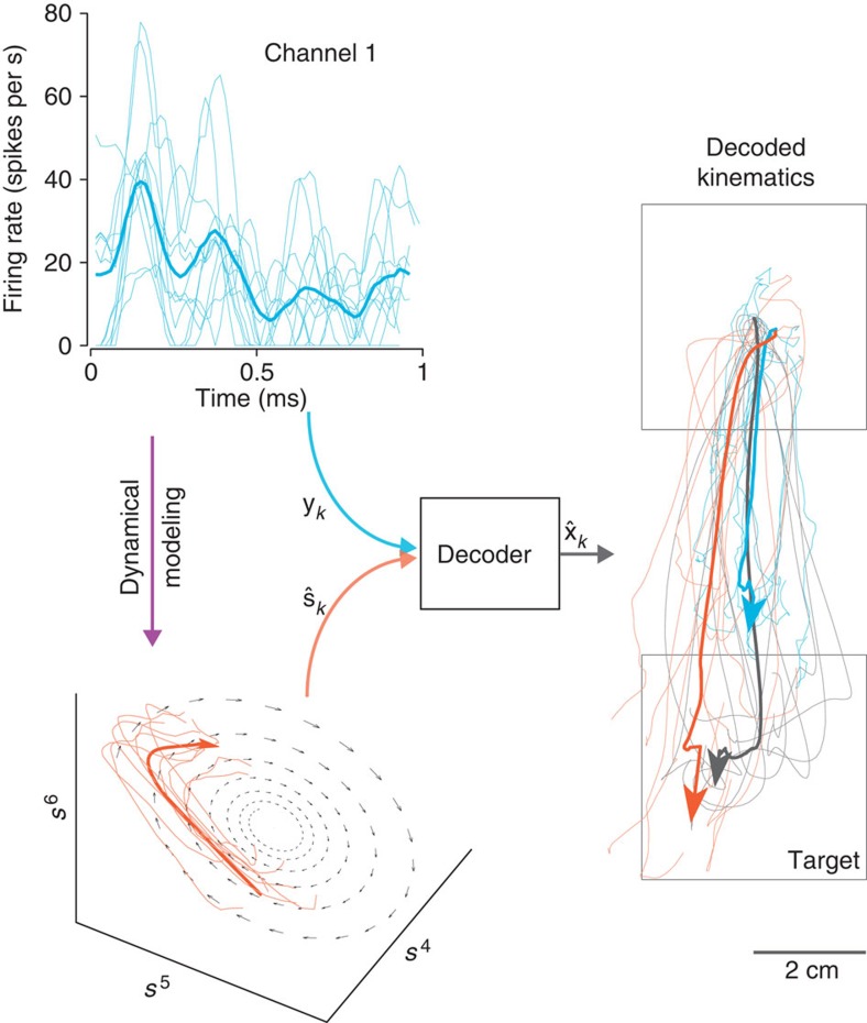
A decode algorithm takes neurally derived observations and outputs decoded kinematics, . Most BMI systems decode using noisy neural observations, y_k, which comprise the single-trial spike counts of the neural data. This data (smoothed) is shown for a single channel, where the light blue traces denote the single-trial neural observations when a monkey intended to reach downwards. The bolded trace is the firing rate averaged over trials (relative to the start of the trial), or peristimulus time histogram. To the right of the decoder block, the black traces denote the true path of the cursor for trials where the monkey reaches from the upper square target to the lower square target (where both squares are 4 × 4 cm). The bolded trajectory is the average path of the cursor across single-trials. The offline reconstructions using the dynamical neural state result in a superior offline decode when compared with using the the non-dynamical binned spike counts.

Figure 5. Graphical representation of decoder algorithms.

(a) A graphical representation of a proposed neural dynamical filter, modelling the dynamics of the neural state (s_k). The neural state propagates through time obeying modelled dynamics, at each point in time generating both the kinematics (x_k) and the observed neural data (y_k). (b) Graphical representation of the linear dynamical system underlying kinematic-state Kalman filters, where the kinematics (x_k) are related through a linear dynamical update rule, and are causal to neural observations (y_k). There is no temporal structure modelled in the neural activity. We also note that this model is of opposite causality to that of a, since kinematics are generative of the neural activity rather than neural population activity (reflected by the neural state) being generative of kinematics.

Figure 6. Online experimental performance of various decoders.

We calculated the mean bitrates (error bars denote s.e.m. across experimental blocks) normalized by the bitrate of the highest performing decoder. More details on statistics and how we calculated mean bitrates are in the Methods and Supplementary Tables 2 and 3. (a) On the x axis, ‘X SD' refers to an optimal linear estimator (OLE) decoder where the neural data were smoothed by a causal Gaussian kernel with a s.d. of X  ms. The bitrate of the neural dynamical filter (NDF) is 31% higher than the best OLE with Gaussian smoothing (P<0.01, paired t-test). The absolute performance of each decoder is denoted by the text in each bar. The performance was evaluated across 29 experimental blocks (except for OLE000 that was evaluated on 25 of the 29 experimental blocks due to monkey motivation). (b) The NDF achieved a bitrate 47% higher than the kinematic-state Kalman filter (KKF; P<0.01, paired t-test). 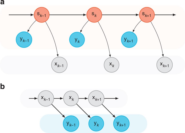Differences in performance of the NDF across decoder comparisons can be attributed to monkey motivation as well as performance variability across weeks. For example, when a decoder performs poorly, such as the KKF, the performance of the NDF in these paired data sets tend to be lower. The performance was evaluated across 22 experimental blocks. (c) The NDF achieved a bitrate 16% higher than the WF (P<0.01, paired t-test). The performance was evaluated across 21 experimental blocks. (d) The NDF achieved a bitrate 83% higher than the best OLE with Gaussian smoothing (P<0.01, paired t-test). The performance was evaluated across 20 experimental blocks (except for OLE000 and OLE050 that were evaluated on 6 and 17 of the 20 experimental blocks, respectively). (e) The NDF achieved a bitrate 61% higher than the KKF (P<0.01, paired t-test). The performance was evaluated across 18 experimental blocks. (f) The NDF achieved a bitrate 13% higher than the WF (P<0.01, paired t-test). The performance was evaluated across 21 experimental blocks. (g–i) For Monkey J, the histograms of target acquire times for each decoder is shown (mean data in Supplementary Table 2). In the inset, the physical workspace of a 6 × 6 grid of targets is shown, and the target acquisition success rate in the workspace is represented by a heat map. (j–l) Same as g–i but for Monkey L.

References

-
- Shenoy K. V., Sahani M. & Churchland M. M. Cortical control of arm movements: a dynamical systems perspective. Annu. Rev. Neurosci. 36, 337–359 (2013) . - PubMed
- Briggman K. L. & Kristan W. B. Jr. Multifunctional pattern-generating circuits. Annu. Rev. Neurosci. 31, 271–294 (2008) . - PubMed
- Petreska B. et al.. Dynamical segmentation of single trials from population neural data. Adv. Neural Inf. Process Syst. 24, 756–764 (2011) .
- Rokni U. & Sompolinsky H. How the brain generates movement. Neural Comput. 24, 289–331 (2012) . - PubMed
Publication types
MeSH terms
Grants and funding
LinkOut - more resources
Full Text Sources
Other Literature Sources